# load packages
library(brms)22 {brms}
In most cases, we do not have to write our own Stan code, because the {brms} package can do that for us. The brm() function in the {brms} takes glm()-like arguments, and writes accurate and fast Stan code. If brm() works for your application, you should much prefer it to writing your on Stan models. It will (probably) be faster and is less like to have errors.
{brms} offers very flexible options for specifying your models and works with {marginaleffects}. We can use it for almost any application, though for simple lm() or glm() fits, it isn’t needed.
See ?brms::brm for the details. There are numerous tutorials available for specific models.
22.1 The turnout example
Here’s the syntax for our ususal logistic regression model.
# load only the turnout data frame and hard-code rescaled variables
turnout <- ZeligData::turnout  |>
  mutate(across(age:income, arm::rescale, .names = "rs_{.col}"))

# build model frame and design matrices
f  <- vote ~ rs_age + rs_educate + rs_income + race

# fit model with glm()
fit_glm <- glm(f, data = turnout, family = binomial)

# fit model with brm()
fit_brm_rstan <- brm(f, data = turnout, family = bernoulli,
           chains = 10, cores = 10)

# fit model with brm() via cmdstan!
fit_brm_cmdstanr <- brm(f, data = turnout, family = bernoulli,
           chains = 10, cores = 10,
           backend = "cmdstanr")
glm() and brm() obtain the same estimates.1
1 The two are not mathematically equal, but they are very close in practice. Outside of cases where maximum likelihood fails, it is rare that a Bayesian estimate or interval differs from the ML estimate or interval.
Code
library(modelsummary)

normalize_terms <- function(x) {
  x <- sub("^b_", "", x)  # brms to glm names
  x <- ifelse(x == "(Intercept)", "Intercept", x)  # unify intercept
  x
}

modelsummary(
  list("glm()" = fit_glm, "brm(); rstan" = fit_brm_rstan, "brm(); cmdstanr" = fit_brm_cmdstanr),
  coef_rename = normalize_terms,
  gof_map = NULL
)| glm() | brm(); rstan | brm(); cmdstanr | |
|---|---|---|---|
| Intercept | 1.058 | 1.062 | 1.062 |
| (0.140) | |||
| rs_age | 0.993 | 0.996 | 0.997 |
| (0.121) | |||
| rs_educate | 1.184 | 1.188 | 1.186 |
| (0.137) | |||
| rs_income | 1.001 | 1.002 | 1.004 |
| (0.154) | |||
| racewhite | 0.251 | 0.248 | 0.251 |
| (0.146) | |||
| Num.Obs. | 2000 | 2000 | 2000 |
| R2 | 0.119 | 0.119 | |
| AIC | 2034.0 | ||
| BIC | 2062.0 | ||
| Log.Lik. | -1011.991 | ||
| ELPD | -1017.1 | -1017.2 | |
| ELPD s.e. | 23.0 | 23.0 | |
| LOOIC | 2034.2 | 2034.5 | |
| LOOIC s.e. | 46.1 | 46.0 | |
| WAIC | 2034.2 | 2034.5 | |
| RMSE | 0.41 | 0.41 | 0.41 |
And {brms} plays very nicely with {marginaleffects}.
library(marginaleffects)

# compute first different
comparisons(fit_brm_cmdstanr, variables = list(rs_age = c(-0.5, 0.5)),
            newdata = datagrid(grid_type = "mean_or_mode"))
 Estimate 2.5 % 97.5 %
    0.167 0.128  0.205

Term: rs_age
Type: response
Comparison: 0.5 - -0.5
# compute and plot expected values (i.e., predicted probabilities)
p <- predictions(fit_brm_cmdstanr, variables = list(rs_age = seq(-1, 1, by = 0.1)),
newdata = datagrid(grid_type = "mean_or_mode"))
ggplot(p, aes(x = rs_age, y = estimate, ymin = conf.low, ymax = conf.high)) +
geom_ribbon(fill = "grey") +
geom_line()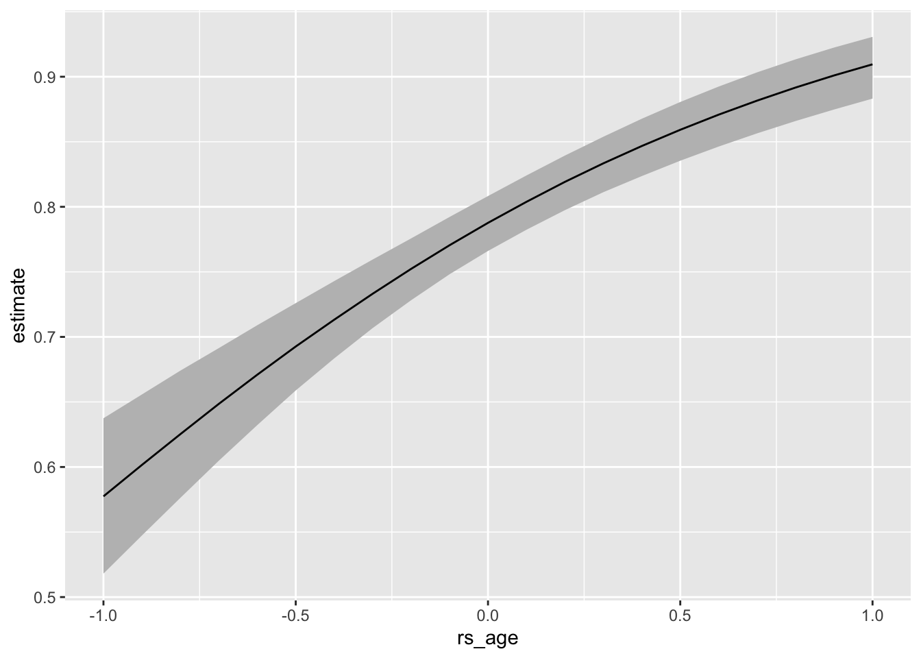
22.2 The flexibility of MCMC and brm()
22.2.1 Modeling “smooth” relationships
To illustrate the power of MCMC and brm(), we can imagine fitting a smooth curve for age. The details are not important for now, but this isn’t an easy task in our usual framework. But it’s straightfoward with Bayesian MCMC via brm().
# smooth relationship between age and voting--notice the s()
f  <- vote ~ s(rs_age) + rs_educate + rs_income + race
smooth_fit <- brm(f, data = turnout, family = bernoulli,
           chains = 10, cores = 10,
           backend = "cmdstanr")
# compute and plot expected values (i.e., predicted probabilities)
p <- predictions(smooth_fit, variables = list(rs_age = seq(-1, 1, by = 0.1)),
newdata = datagrid(grid_type = "mean_or_mode"))
ggplot(p, aes(x = rs_age, y = estimate, ymin = conf.low, ymax = conf.high)) +
geom_ribbon(fill = "grey") +
geom_line()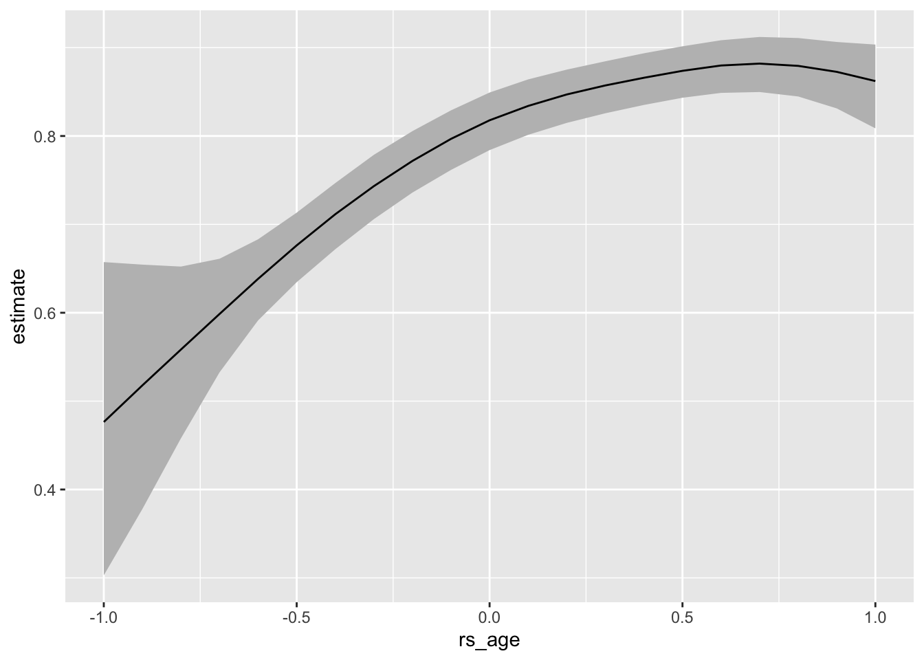
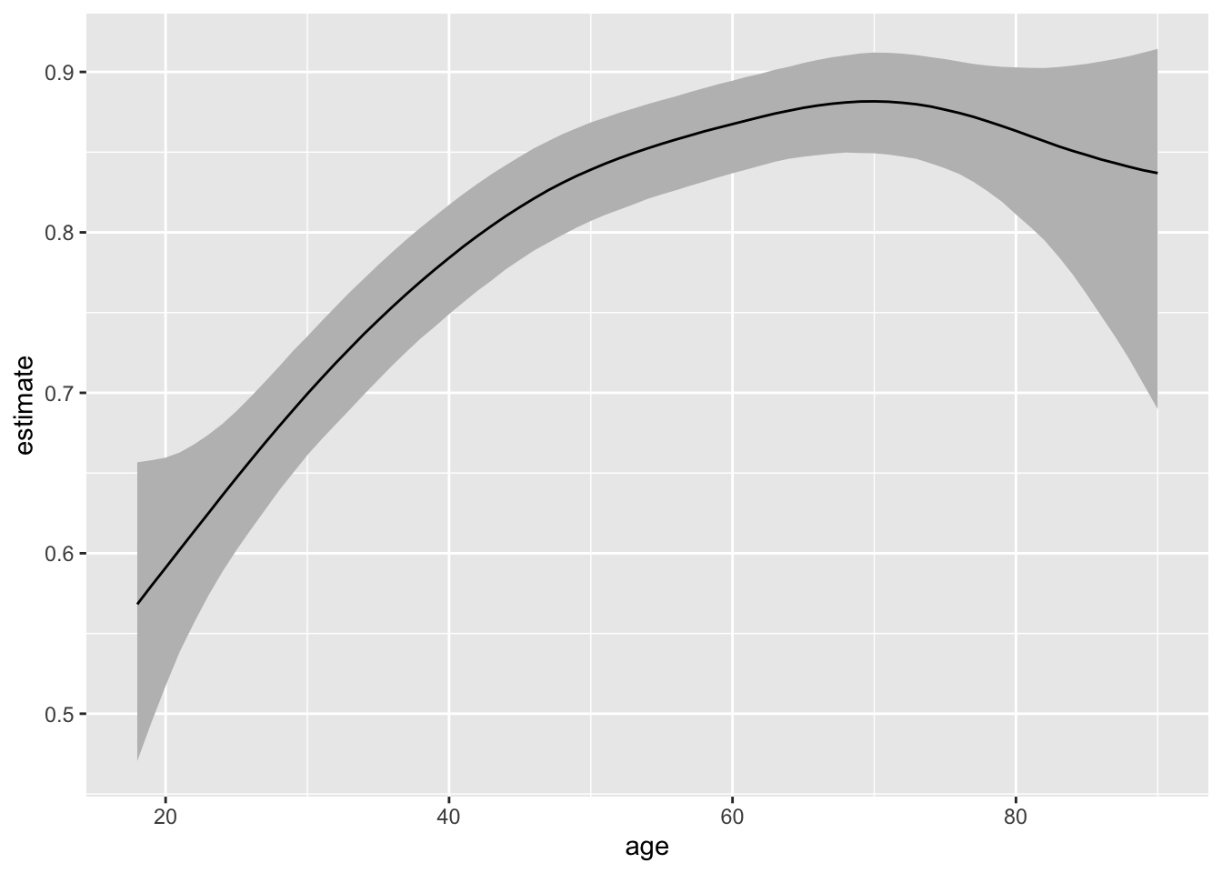
22.2.2 Awkwardly scaled variables
Also, brm() has no trouble with the variables on their original scales. The original scales poses a insurmountable hurdle for our metrop() sampler.
# smooth relationship between age and voting--notice the s()
f  <- vote ~ s(age) + educate + income + race
smooth_fit <- brm(f, data = turnout, family = bernoulli,
           chains = 10, cores = 10,
           backend = "cmdstanr")
# compute and plot expected values (i.e., predicted probabilities)
p <- predictions(smooth_fit, variables = list(age = seq(18, 90, by = 1)),
newdata = datagrid(grid_type = "mean_or_mode"))
ggplot(p, aes(x = age, y = estimate, ymin = conf.low, ymax = conf.high)) +
geom_ribbon(fill = "grey") +
geom_line()