6 Fisher Information Matrix
We can easily use the log-likelihood function to obtain point estimates. It turns out, though, that the same log-likelihood function contains information that we can use to estimate the precision of those estimates as well.
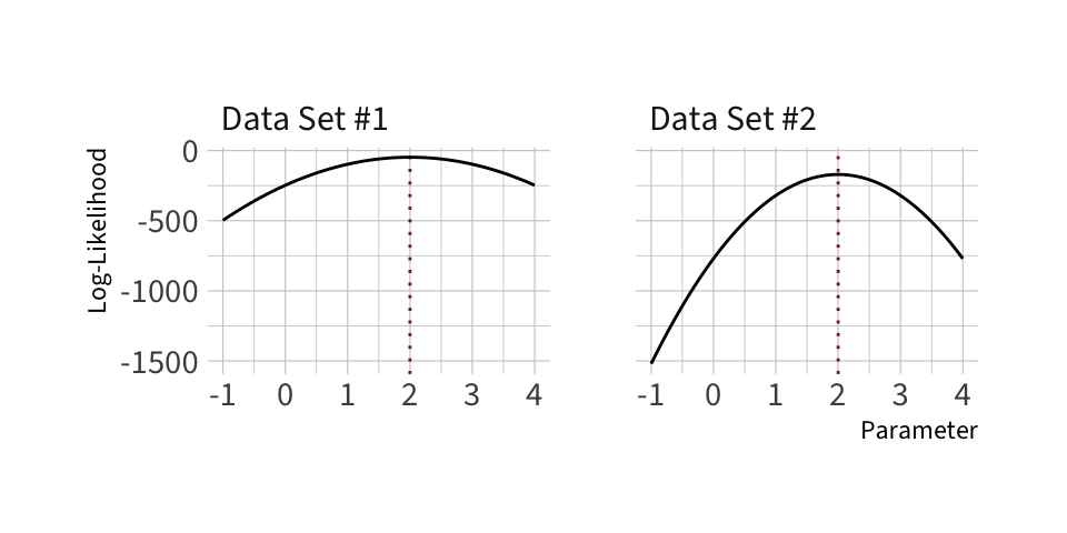
As an example, consider the following two log-likelihood functions:
Which of these two log-likelihood functions do you think provides a more precise estimate?
Note: These likelihoods are from a normal model with unknown mean. I simulated 100 observations for \(y_1\) and 300 observations for \(y_2\). (I centered the data so the sample means both occurred exactly at 2).
Key Idea: We can use the curvature around the maximum likelihood estimate to get a sense of the uncertainty.
What quantity tells us about the amount of curvature at the maximum? The second derivative. As the second derivative becomes more negative (its magnitude increases), the curvature goes up. As the curvature goes up, the uncertainty goes down.
6.1 Example: Stylized Normal
In this example, we examine curvature for a single-parameter model.
To develop our intuition about “curvature” and confidence intervals, I analyze the Stylized Normal Model (\(\sigma = 1\)). Here, we model the data as a normal distribution with \(\mu\) unknown (and to be estimated), but \(\sigma = 1\) (known; not estimated). That is, \(y \sim N(\mu, 1)\).
\[ \begin{aligned} \ell(\mu) &= -\tfrac{N}{2}\log(2\pi) - \tfrac{1}{2}\sum_{i = 1}^N (y_i - \mu)^2\\ \dfrac{\partial \ell(\mu)}{\partial \mu} &= \sum_{i = 1}^N (y_i - \mu) = \sum y_i - N\mu\\ \dfrac{\partial^2 \ell(\mu)}{\partial \mu^2} &= - N \end{aligned} \]
Facts:
- As \(N\) increases, \(\dfrac{\partial^2 \ell(\mu \mid y)}{\partial \mu^2}\) becomes more negative.
- As the magnitude of \(\dfrac{\partial^2 \ell(\mu \mid y)}{\partial \mu^2}\) increases, the curvature increases.
- As the curvature increases, the uncertainty decreases.
Wouldn’t it be really nice if we could use \(\dfrac{\partial^2 \ell(\mu)}{\partial \mu^2}\) to estimate the standard error?
It turns out that this quantity is a direct, almost magically intuitive estimator of the standard error.
6.2 Theory
Definition 6.1 (Fisher Information) For a model \(f(y \mid \theta)\) with log-likelihood \(\ell(\theta) = \sum_{i=1}^N \log f(y_i \mid \theta)\), the expected information is defined as \(\mathcal I(\theta) = -\mathbb E_\theta\!\left[\nabla^2 \ell(\theta)\right]\).
In practice, we often use the observed information, given by the negative Hessian of the log-likelihood at the ML estimate \(\mathcal I_{\text{obs}}(\hat\theta) = -\nabla^2 \ell(\hat\theta)\).
There’s an important theoretical distinction between the expected and observed information. The expected Fisher information \(\mathcal I(\theta) = \mathbb E_\theta[-\nabla^2 \ell(\theta)]\) is the expected curvature of the log-likelihood under the model. In contrast, the observed information \(\mathcal I_{\text{obs}}(\hat\theta) = -\nabla^2 \ell(\hat\theta)\) uses the curvature at the ML estimate \(\hat{\theta}\) from a particular sample. Under standard regularity conditions, both lead to the same large-sample variance: \(\mathcal I_{\text{obs}}(\hat\theta) \overset{p}{\to} \mathcal I(\theta)\) and \(\widehat{\operatorname{Var}}(\hat\theta) \approx \mathcal I_{\text{obs}}(\hat\theta)^{-1} \approx \mathcal I(\theta)^{-1}\). And in many examples, they are numerically identical. In some weird cases, the expected information is “more robust.” In these notes, I use the observed information to make the curvature↔︎uncertainty link concrete and intuitive.
Recall that \(\nabla\) denotes the gradient vector of first derivatives of the log-likelihood with respect to the parameters,
\[
\nabla \ell(\theta) \;=\;
\begin{bmatrix}
\dfrac{\partial \ell}{\partial \theta_1} \\
\dfrac{\partial \ell}{\partial \theta_2} \\
\vdots \\
\dfrac{\partial \ell}{\partial \theta_k}
\end{bmatrix}.
\]
The Hessian \(\nabla^2\) is the square matrix of second derivatives,
\[\small
\nabla^2 \ell(\theta) \;=\;
\begin{bmatrix}
\dfrac{\partial^2 \ell}{\partial \theta_1^2} &
\dfrac{\partial^2 \ell}{\partial \theta_1 \partial \theta_2} & \cdots & \dfrac{\partial^2 \ell}{\partial \theta_1 \partial \theta_k} \\
\dfrac{\partial^2 \ell}{\partial \theta_2 \partial \theta_1} &
\dfrac{\partial^2 \ell}{\partial \theta_2^2} & \cdots & \dfrac{\partial^2 \ell}{\partial \theta_2 \partial \theta_k} \\
\vdots & \vdots & \ddots & \vdots \\
\dfrac{\partial^2 \ell}{\partial \theta_k \partial \theta_1} &
\dfrac{\partial^2 \ell}{\partial \theta_k \partial \theta_2} & \cdots & \dfrac{\partial^2 \ell}{\partial \theta_k^2}
\end{bmatrix}.
\] These gradient and Hessian objects are the matrix calculus tools needed to define Fisher information.
Theorem 6.1 (Asymptotic Normality of ML Estimators) Let \(y_1,\dots,y_N\) be iid from a model \(f(y \mid \theta)\) with true parameter \(\theta\). Suppose the regularity conditions in Theorem 1.1 hold and the Fisher information matrix \(\mathcal I(\theta)\) is finite and positive definite. Then the maximum likelihood estimator \(\hat\theta\) is asymptotically normal \(\hat\theta \overset{a}{\sim} \mathcal N\big(\theta, \mathcal I(\theta)^{-1}\big)\).
This is an important result, because it tells us the location (i.e., \(\theta\)), variability (i.e., \(\mathcal I(\theta)^{-1}\)), and shape (i.e., normal) of the sampling distribution asymptotically. These asymptotic results tend to be good approximations in practice.
Theorem 6.2 (Asymptotic Variance of ML Estimators) Under the conditions of Theorem 6.1, the covariance of the maximum likelihood estimator is well-approximated by the inverse Fisher information $ () ;; I()^{-1}$.
In practice, we replace the unknown \(\theta\) with the maximum likelihood estimate and use the observed information \(\widehat{\operatorname{Var}}(\hat\theta) \;\approx\; \big[-\nabla^2 \ell(\hat\theta)\big]^{-1}\).
For a single parameter \(\theta\), this reduces to \(\widehat{\operatorname{Var}}(\hat\theta) \;\approx\; \left[\,-\,\dfrac{\partial^2 \ell(\theta)}{\partial \theta^2}\Bigg|_{\theta=\hat\theta}\right]^{-1}\).
Approximations via asymptotics
We should be careful here. The results above are asymptotic. As the sample size grows, the variance of \(\hat{\theta}\) eventually converges to \(\left[\left. - \dfrac{\partial^2 \ell(\theta)}{\partial \theta^2}\right| _{\theta = \hat{\theta}}\right] ^{-1}\). However, “eventually gets close” does not imply “is close” for a finite sample size. However, we are usually safe to treat asymptotic results as good approximations.
This means that we can estimate the SE as follows:
- Find the second derivative (or Hessian if multiple parameters) of the log-likelihood.
- Evaluate the second derivative at the maximum (\(\theta = \hat{\theta}\)).
- Find the inverse. (That’s an estimate of the variance.)
- Take the square root.
\[ \widehat{\text{SE}}(\hat{\theta}) = \sqrt{\left[\left. - \dfrac{\partial^2 \ell(\theta)}{\partial \theta^2}\right| _{\theta = \hat{\theta}}\right] ^{-1}} \]
If we continue the stylized normal example, we have the following.
\[ \begin{equation*} \dfrac{\partial^2 \ell(\mu \mid y)}{\partial \mu^2} = - N ~{\color{purple}{\Longrightarrow}}~ \left[\left. - \dfrac{\partial^2 \ell(\mu \mid y)}{\partial \mu^2}\right| _{\mu = \hat{\mu}}\right] ^{-1} = \dfrac{1}{N} \approx \widehat{\operatorname{Var}}(\hat{\mu}) \end{equation*} \]
And then
\[ \begin{equation*} \widehat{\text{SE}}(\hat{\mu}) \approx \sqrt{\dfrac{1}{N}} \end{equation*} \]
Does this answer make sense? What is the classic standard error of the mean when taking a random sample from a population? Hint: It’s \(\text{SE}[\operatorname{avg}(y)] = \sigma/\sqrt{N}\). In this case, the “population SD” is \(\sigma = 1\), as assumed by the stylized normal model.
6.3 Curvature in Multiple Dimensions
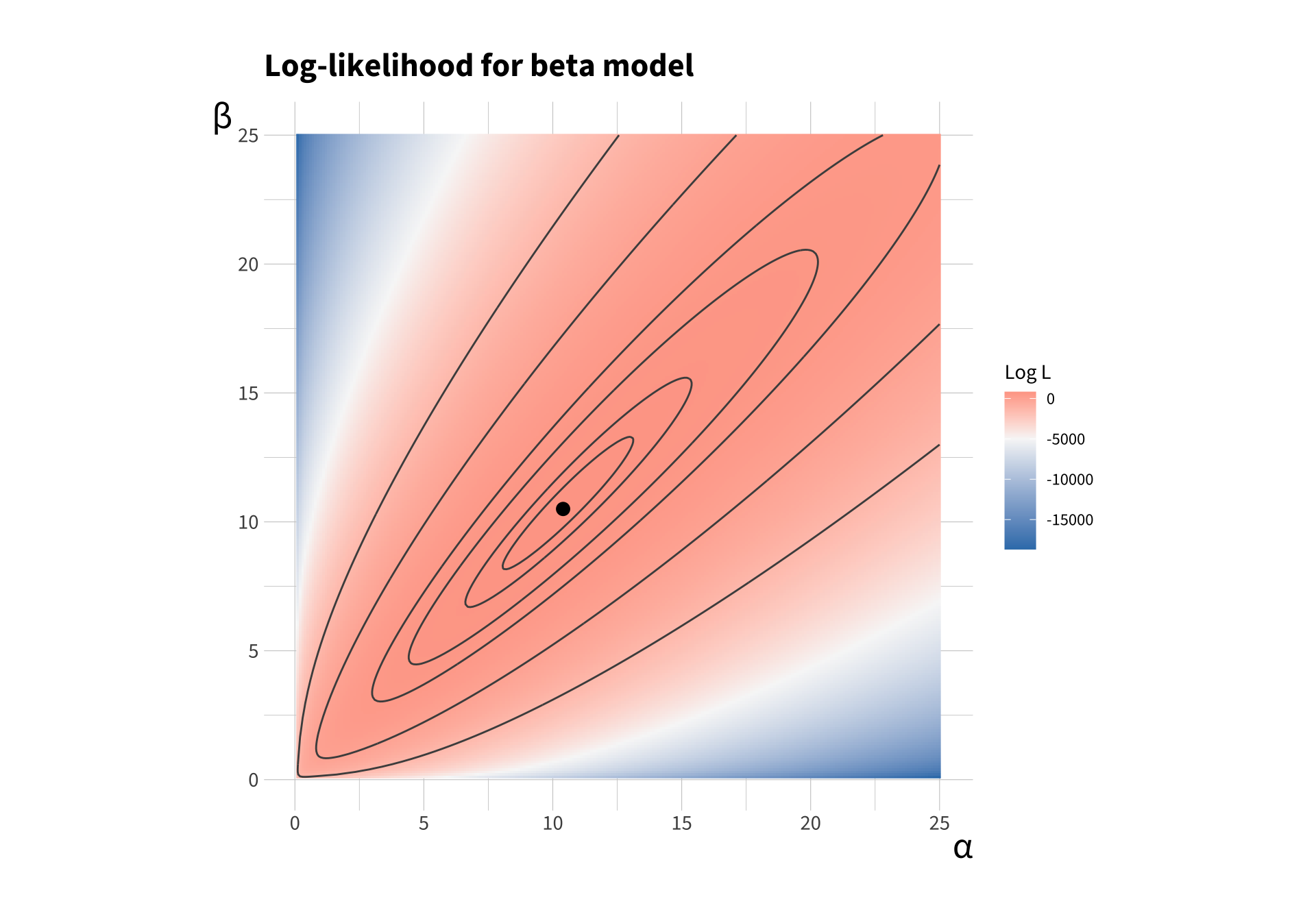
To add multiple dimensions, let’s consider the beta model. Our goal is to estimate \(\alpha\) and \(\beta\). The key is that we have multiple (i.e., two) parameters to estimate.
It’s a bit trickier to think about curvature in multiple dimensions. Instead of a second derivative like we have in a single dimension, we have Hessian matrix in multiple dimensions.
Here’s what the log-likelihood function might look like for a given data set. This is a raster and contour plot. The contour lines connect parameter combinations with the same log-likelihood. The color shows the log-likelihood — larger log-likelihoods are red and small log-likelihoods are blue.
To make more sense of this, here’s a version you can rotate.