Previously, we looked at the Metropolis algorithm and saw how it could generate samples from an unnormalized posterior. Metropolis is general and powerful, but requires many iterations to explore the posterior and careful tuning of proposal distributions.
In this chapter, we look at Stan, a modern and general-purpose platform for Bayesian inference (Carpenter et al. 2017). Stan automates the process of sampling from complex posterior distributions using a hyper-optimized version of Hamiltonian Monte Carlo (HMC) (Neal 2011), which is itself a form of Markov Chain Monte Carlo (MCMC). Betancourt (2017) provides a nice introduction to HMC.
Carpenter, Bob, Andrew Gelman, Matthew D. Hoffman, Daniel Lee, Ben Goodrich, Michael Betancourt, Marcus Brubaker, Jiqiang Guo, Peter Li, and Allen Riddell. 2017. “Stan: A Probabilistic Programming Language.”Journal of Statistical Software 76 (1): 1–32. https://doi.org/10.18637/jss.v076.i01.
Neal, Radford M. 2011. “MCMC Using Hamiltonian Dynamics.” In Handbook of Markov Chain Monte Carlo, edited by Steve Brooks, Andrew Gelman, Galin Jones, and Xiao-Li Meng, 113–62. Chapman; Hall/CRC. https://doi.org/10.1201/b10905-6.
Hoffman, Matthew D., and Andrew Gelman. 2014. “The No-u-Turn Sampler: Adaptively Setting Path Lengths in Hamiltonian Monte Carlo.”Journal of Machine Learning Research 15: 1593–623. https://jmlr.org/papers/v15/hoffman14a.html.
Stan handles nearly all the details automatically: step sizes, trajectory lengths, tuning, and adaptation (Hoffman and Gelman 2014). This allows the user to focus on the model itself.
Before Stan, Bayesian modeling in R was typically done using BUGS or JAGS, which relied on Gibbs sampling and Metropolis-within-Gibbs updates. These samplers were intuitive and easy to use but often slow to converge, especially for correlated or high-dimensional parameters.
Stan was designed to overcome these limitations. It uses gradients of the log-posterior to navigate the parameter space more efficiently, improving both speed and accuracy.
We’ll assume weakly informative priors (i.e., variance = 25). Because the scale of the variables affects the interpretation of the priors, it’s common to rescale variables to have a common scale (e.g., SD of 0.5, SD of 1, or range of 1). For example, a prior with an SD of 5 is more or less informative depending on whether income is dollars or thousands of dollars—the coefficient is 1000x larger in the latter case.
\[
\beta \sim \mathcal{N}(0, 5^2 I).
\]
21.2 Stan Model
To use Stan, we need to represent the model in Stan’s syntax.1
1 Stan is a declarative modeling language: you describe the data you have, the parameters you don’t know, and the probabilistic relationships (priors and likelihood) that connect them. Stan then draws samples from the posterior using HMC.
parameters { ... } Unknowns to infer (e.g., vector[K] beta;, real<lower=0> sigma;). Put constraints that reflect the parameter’s support.
model { ... } Priors and likelihood live here. Use sampling statements (theta ~ normal(0,1);)
There are other blocks you can use as well.
As an example, the model below is how we can represent our logit model in Stan. We should save this text file as logit.stan in our project directory.
The Stan model mirrors the math closely.
# data blockdata {int<lower=0> N; // rows in design matrixint<lower=1> K; // colummns in design matrixarray[N] int<lower=0, upper=1> y; // binary outcomematrix[N, K] X; // design matrix}# parameters blockparameters {vector[K] beta; // logit coefficients}# model blockmodel { beta ~ normal(0, 5); // n(0, 5) prior for each beta y ~ bernoulli_logit(X * beta); // logistic regression likelihood}
21.3 Data for Stan
We can use the same turnout data and formula from the Metropolis chapter.
# load only the turnout data frameturnout <- ZeligData::turnout |># hard code rescaled variables, because comparisons doesn't like them in the formula for some reason I don't understandmutate(across(age:income, arm::rescale, .names ="rs_{.col}")) |>glimpse()
Inference for Stan model: anon_model.
4 chains, each with iter=3000; warmup=1000; thin=1;
post-warmup draws per chain=2000, total post-warmup draws=8000.

        mean se_mean   sd  2.5%  25%  50%  75% 97.5% n_eff Rhat
beta[1] 1.06       0 0.14  0.78 0.96 1.06 1.16  1.34  4596    1
beta[2] 1.00       0 0.12  0.77 0.92 1.00 1.08  1.24  6057    1
beta[3] 1.19       0 0.14  0.92 1.10 1.19 1.28  1.46  5686    1
beta[4] 1.00       0 0.15  0.71 0.90 1.00 1.11  1.31  6289    1
beta[5] 0.25       0 0.15 -0.03 0.16 0.25 0.35  0.54  4763    1

Samples were drawn using NUTS(diag_e) at Wed Oct  8 12:51:46 2025.
For each parameter, n_eff is a crude measure of effective sample size,
and Rhat is the potential scale reduction factor on split chains (at
convergence, Rhat=1).
21.5cmdstanr
The {cmdstanr} package interfaces with the CmdStan engine outside R. It compiles quickly and provides clear diagnostic output. This is slightly more tedious to set up and maintain, but is preferred to {rstan}.
Both interfaces fit the same model and return similar results. Either is fine! I recommend {cmdstanr}, though it is slightly more work to get started.
Feature
rstan
cmdstanr
Compilation
Inside R
External CmdStan executable
Speed
Slower
Faster (cached binaries)
Debugging
Less transparent
Easier (visible console output)
Recommendation for new users
✅ Works fine
✅ Preferred
21.6 Diagnostics
Stan reports two essentials:
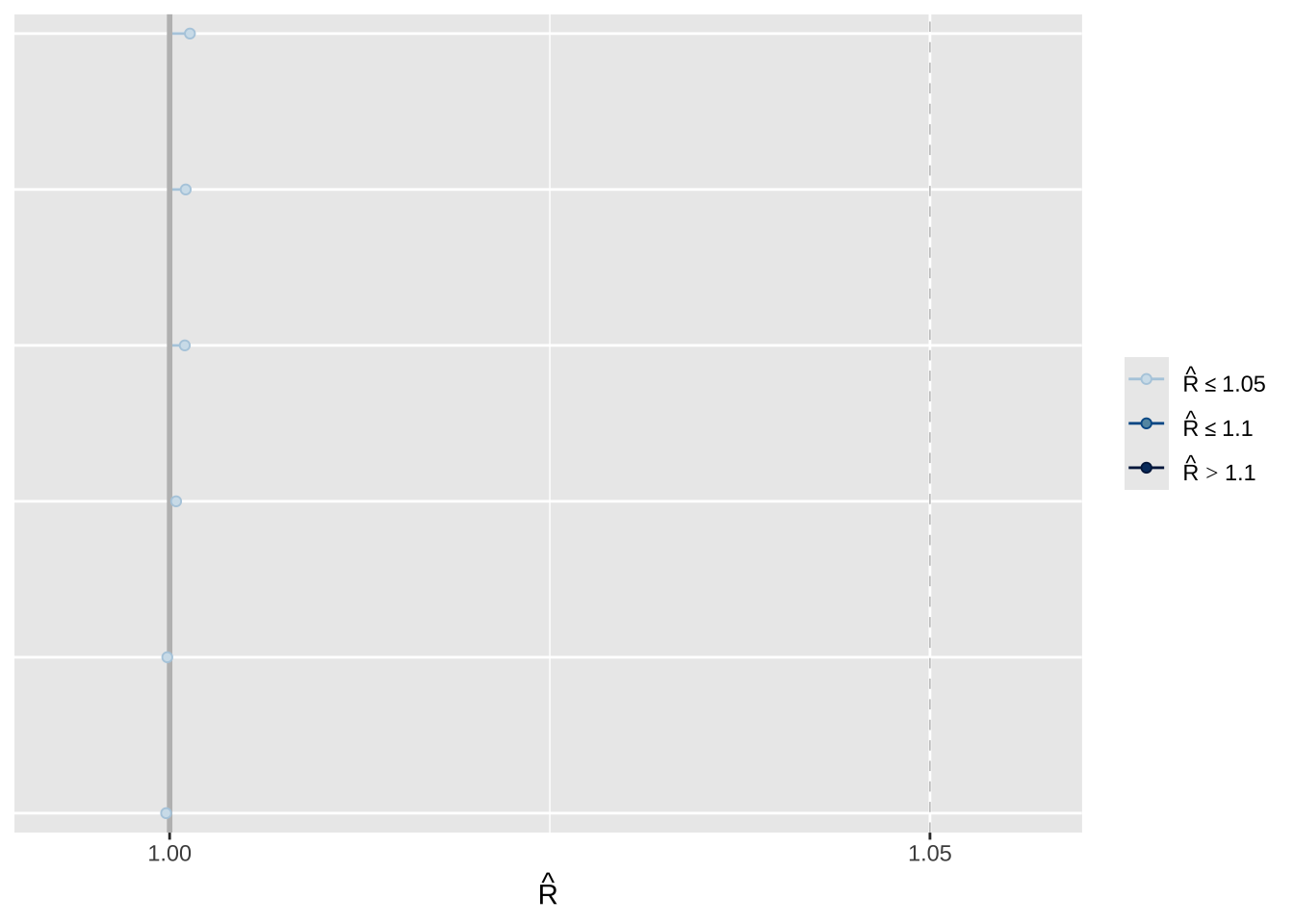
\(\hat{R}\): near 1 indicates convergence across chains.
Effective Sample Size (ESS): how much independent information is in the draws.
The print() methods make these easy to find, but we can also compute them directlyAs a rule of thumb, check \(\hat{R} < 1.01\) and ESS > 2,000.
library(posterior)draws_beta <- fit_cmd$draws(variables ="beta") # draws arrayrhat(draws_beta)
[1] 1.18
ess_bulk(draws_beta)
[1] 5.91
ess_tail(draws_beta)
[1] 12
21.6.1 {bayesplot}
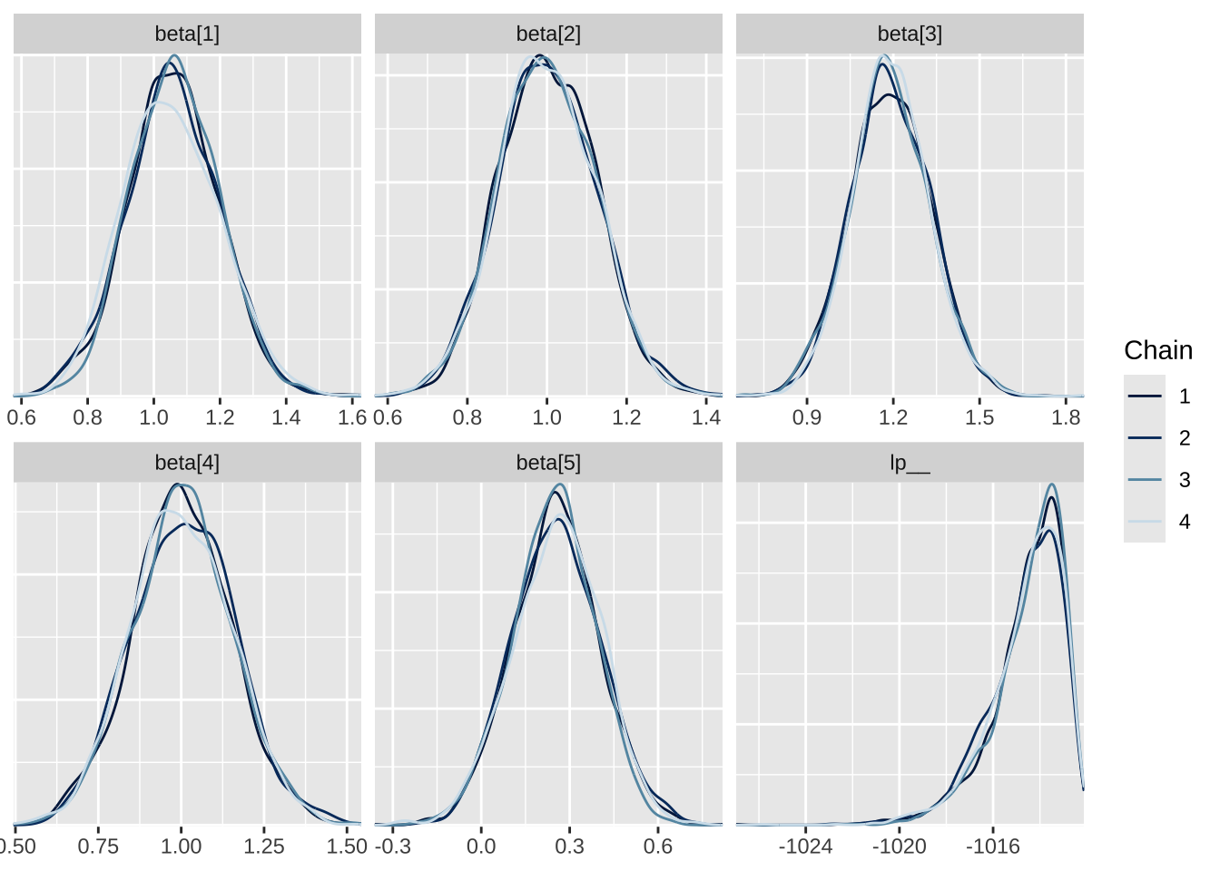
The {bayesplot} packages offers many useful functions for visualizing the simulations. There are three examples below, but there are many more useful tools in {bayesplot}. Again, the documentation is excellent.
# load packageslibrary(bayesplot)# densities of parameters by chainmcmc_dens_overlay(fit_rstan)
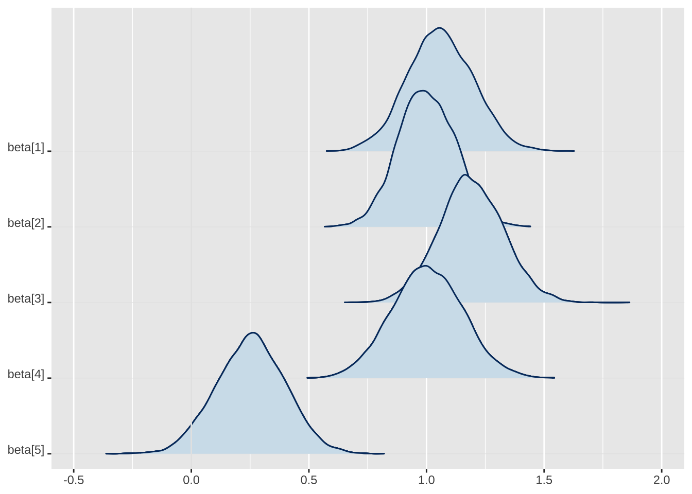
# ridges plot of densities of parametersmcmc_areas_ridges(fit_rstan, regex_pars ="beta")
# r-hatmcmc_rhat(rhat(fit_rstan))
21.6.2 {ShinyStan}
The ShinyStan app provides an interactive dashboard for convergence diagnostics, traceplots, divergences, and posterior summaries.
# launching a GUI is interactive; keep this non-evaluated by defaultlibrary(shinystan)# for rstanlaunch_shinystan(fit_rstan)# for cmdstanr: convert to a stanfit first, then launchsf <- rstan::read_stan_csv(fit_cmd$output_files())launch_shinystan(sf)
You can inspect \(\hat{R}\), ESS, and visual diagnostics interactively without additional coding.
21.7 Quantities of Interest
We have simulations of \(\beta\). We can summarize these with means, medians, SDs, quantiles, etc. The {posterior} package offers many useful function for working with the simulations from {rstan} and {cmdstanr}. Again, the documentation for {posterior} is excellent. Here, we can use the as_draws_matrix() function to extract the MCMC samples from fit_rstan.
# put the simulations of the coefficients into a matrixbeta_tilde_raw <- posterior::as_draws_matrix(fit_rstan, regex_pars ="beta")head(beta_tilde_raw)
To compute a first difference, transform draws using the invariance principle.
# make X_loX_lo <-cbind("constant"=1, # intercept"rs_age"=-0.5, # 1 SD above avg -- see ?arm::rescale"rs_educate"=0,"rs_income"=0,"white"=1# white indicator = 1 )# make X_hi by modifying the relevant value of X_loX_hi <- X_loX_hi[, "rs_age"] <-0.5# 1 SD below avg# function to compute first differencefd_fn <-function(beta, hi, lo) { beta <-as.vector(beta) # to prevent column/row confusionplogis(hi%*%beta) -plogis(lo%*%beta)}# transform simulations of coefficients into simulations of first-difference# note 1: for clarity, just do this one simulation at a time,# note 2: i indexes the simulationsfd_tilde <-numeric(nrow(beta_tilde)) # containerfor (i in1:nrow(beta_tilde)) { fd_tilde[i] <-fd_fn(beta_tilde[i, ], hi = X_hi, lo = X_lo)}# posterior meanmean(fd_tilde)
[1] 0.167
21.8 Summary
There are three important points to remember.
Stan as modern MCMC
Stan automates MCMC using a hyper-optimized version of HMC. It efficiently samples from posteriors that are otherwise difficult to explore.
Interfaces
Both rstan and cmdstanr run the same Stan model. They differ mainly in compilation method and speed.
Diagnostics and Visualization
Always check \(\hat{R}\) and ESS to ensure convergence. ShinyStan makes it easy to explore diagnostics interactively. summary() and print() methods make these easily available.
Stan generalizes what we learned with the Metropolis algorithm: the logic is the same, but the computation is vastly more efficient.