# install jrnold's package from github# devtools::install_github("jrnold/ZeligData") # just run once# load packageslibrary(tidyverse)# load dataturnout <- ZeligData::turnout # see ?ZeligData::turnout for details# quick lookglimpse(turnout)
And a logit model modeling the binary vote variable as a function of age, educate, income, and race.
# fit logit modelf <- vote ~ age + educate + income + racefit <-glm(f, data = turnout, family = binomial)# print tablemodelsummary::modelsummary(fit, gof_map =NA)
(1)
(Intercept)
-3.034
(0.326)
age
0.028
(0.003)
educate
0.176
(0.020)
income
0.177
(0.027)
racewhite
0.251
(0.146)
These coefficients are not particularly interpretable, so we might want to compute quantities of interest.1
1 In political science, King, Tomz, and Wittenberg (2000) prompted the focus on more interpretable quantities and I often borrow their langauge.
King, Gary, Michael Tomz, and Jason Wittenberg. 2000. “Making the Most of Statistical Analyses: Improving Interpretation and Presentation.”American Journal of Political Science 44: 341–55. http://gking.harvard.edu/files/abs/making-abs.shtml.
We have learned that we can use the invariance property and the delta method as a very general way to compute almost any quantity of interest. The {marginaleffects} package in R exploits this generally to compute many quantities of interest, especially those that are involve \(E(Y)\)–like the commonly used expected value and first difference.
library(marginaleffects)
We’ll focus on two main functions from {marginaleffects}: predictions() and comparisons(), as well as their avg_*() variants. Let’s take a quick look at each.
13.1 Expected value → predictions()
Reminder: expected value = \(E(y \mid X_c)\), where \(X_c\) is a carefully chosen covariate vector.
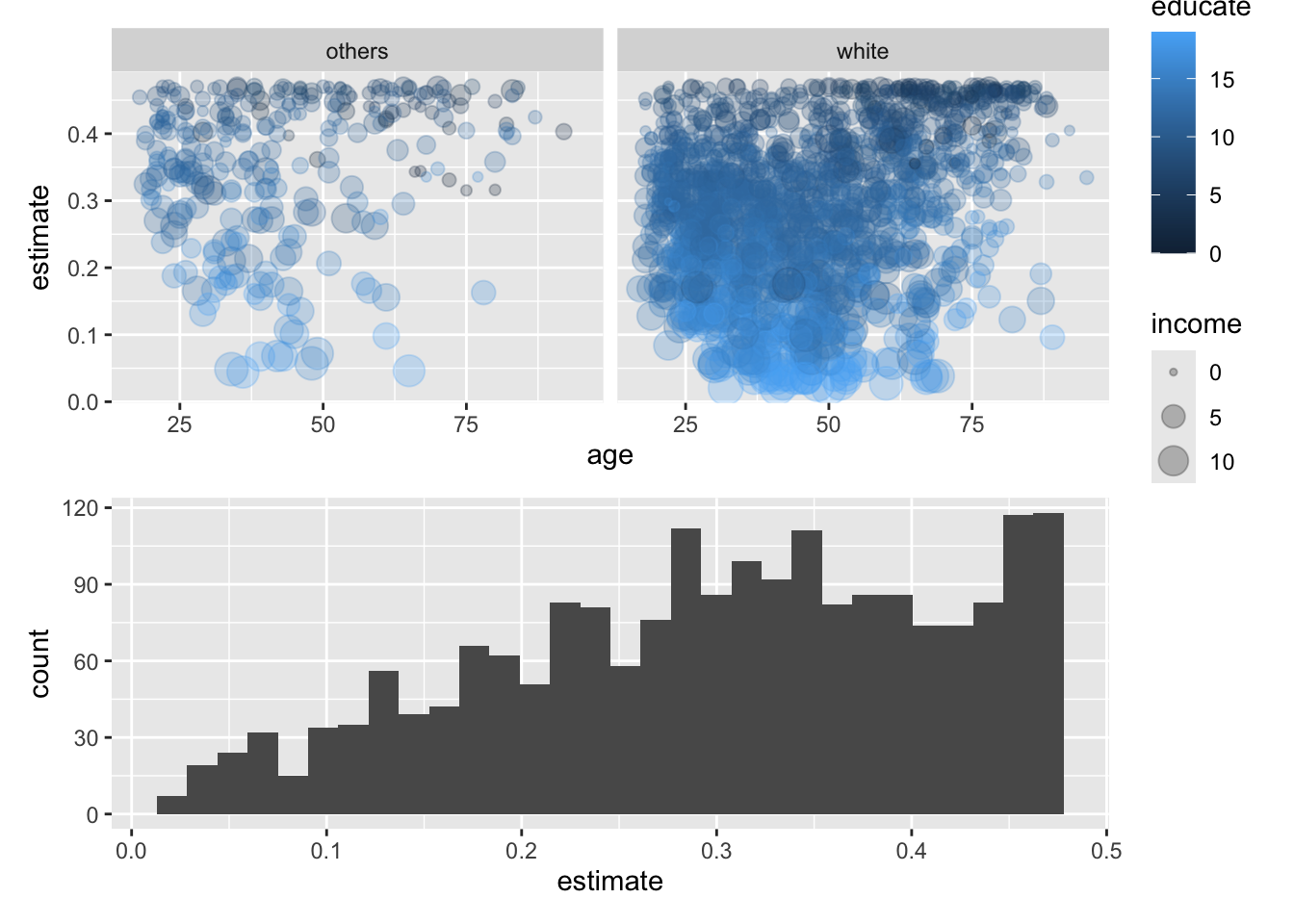
By default, predictions() generates an expected value for every row in the observed dataset. These expected vaues are stored in the estimate column of the output and it includes other commonly used values like the upper and lower bounds of the 95% confidence interval.
Reminder: first difference = \(E(y \mid X_{hi}) - E(y \mid X_{lo})\), where \(X_{hi}\) and \(X_{lo}\) are a carefully chosen covariate vectors that fix on covariate of interest at a high value and low value respectively.
Bcomparisons() computes these first differences
Q: But what variable does it vary by default? A: All of them, one at a time! You’ll usually want to pick one.
Q: And what are the high and low values? A: It depends, but something somewhat reasonable. You’ll almost always want to specify the one you want.
By default, comparisons() computes a first difference varying each variable from a low to a high value, while fixing every other variable to the observed values.
These expected values are stored in the estimate column of the output and it includes other commonly used values like the upper and lower bounds of the 95% confidence interval.
For the numeric variables like age, comparisons() generates a first difference moving age from the observed value age to a high value age + 1. The variable contrast in the output specifies this comparison +1.
For the factor variable race, comparisons() generates a first difference moving race from the reference level to each other factor level. The variable contrast in the output specifies this comparison white - others.
table(fd$term, fd$contrast)
            +1 white - others
  age     2000              0
  educate 2000              0
  income  2000              0
  race       0           2000
Thus, by default, comparisons() gives us a data frame with the observed data repeated several times for several difference first differences. This is a reasonable default behavior, but we’ll almost always want to compute something more specific (and avoid computing things we don’t need).
13.3 Framework
When we call predictions() or comparisons(), we are always making three choices: (1) the quantity we want, (2) the grid of predictor values where we want it, and (3) whether or not to aggregate across units (the idea of “aggregation” is new to us). These choices determine the estimand, and it is important to be explicit in writing and thinking.
Here’s how Arel-Bundock, Greifer, and Heiss (2024) describe these choices:
Arel-Bundock, Vincent, Noah Greifer, and Andrew Heiss. 2024. “How to Interpret Statistical Models Using Marginaleffects for r and Python.”Journal of Statistical Software 111 (9). https://doi.org/10.18637/jss.v111.i09.
Quantity: What is the quantity of interest? Do we want to report a expected value or a comparison of expected values (difference, ratio, derivative, etc.)?
Grid: What predictor values are we interested in? Do we want to report estimates for the units in our dataset, or for hypothetical or representative individuals?
Aggregation: Do we report estimates for every observation in the grid or a global summary?
13.3.1 Quantity
First, we must choose our quantity of interest. Most generally, it can be “whatever we want.” But {marginaleffects} is slightly restrictive.
13.3.1.1 What scale?
First, we must choose the scale of the quantity of interest. For a logistic regression, we almost always want the probability scale (i.e., "response" scale). But we could also choose the linear predictor scale (i.e., "link" scale).
We make this choice with the type= argument:
# probability scale; default; almost always want this onepredictions(fit, type ="response")
Second, we must choose whether we want a prediction or a comparison. We make this choice by using predictions() or comparisons().
Arel-Bundock et al. (2025) define a prediction as:
Predictions are the outcomes predicted by a fitted model on a specified scale for a given combination of values of the predictor variables, such as their observed values, their means, or factor levels.
Borrowing language from King et al. (2000), I refer the {marginaleffects}’s “prediction” as an “expected value.”
They define a comparison as:
Comparisons are functions of two or more predictions. Examples of comparisons include contrasts, differences, risk ratios, odds, lift, etc.
The “first difference” from King et al. (2000) is an example of a comparison–a “difference” in the quote above.
13.3.1.3 What to compare?
Third, if we choose to compare, we need to choose what to compare. This involves two choices.
First, we need to choose a focal variable.
We need to choose a “high” scenario and a “low” scenario.
We specify this focal variable and the scenarios with the variables argument to comparisons(). The variables argument is a list of focal variables and a specification of the high and low values. There are numerous convenient ways to specify the comparisons you want, see ?marginaleffects::comparisons for details. I put a few common examples below for numeric variables.
# focal variable: `age`; high = age + 10; low = agecomparisons(fit, variables =list(age =10)) |>glimpse()
We can also supply our own function \(hi, lo) {...}. I think the percent change \(hi, lo) (hi/lo) - 1) is good. This is also known as “lift” and we can use comparison = "lift" instead.
Next, we need to decide where to compute these predictions or comparisons. In most cases, the values of the non-focal variables matter, so we have to make a choice about these other variables.
By default, predictions() and comparisons() use the observed data, returning one value for each row. However, this isn’t always what we want.
To help us create the grid we want, {marginaleffects} has a powerful datagrid() function.
For example, we can supply newdata = datagrid(type = "mean_or_mode") to predictions(). This computes the prediction for a “typical case” has numeric variables equal to the mean and factor variables equal to their mode.
If we instead supply age = 18:90 to datagrid() then it will create a grid that varies age from 18 to 90 while fixing the other variables at their mean_or_mode.
You can always inspect the output of predictions() to see the grid that you are using.
We can use the same logic with comparisons. We can compute the first difference of a focal variable while systematically varying another variable (e.g., educate or race) and fixing the other variables at their "mean_or_mode".
# first difference of moving age from 18 to 90 for respondents with # 12, 14, and 16 years of educationcomparisons(fit, variables =list(age =c(18, 90)), newdata =datagrid(educate =c(12, 14, 16))) |>glimpse()
# first difference of moving age from 18 to 90 for white respondents # and for non-white respondentscomparisons(fit, variables =list(age =c(18, 90)), newdata =datagrid(race = unique)) |>glimpse()
Finally, we need to decide what to do with the collection of estimates from the grid. For example, by default, comparisons returns a first difference for every row in the data set.
It’s really useful to summarize the heterogeneity of the effects from your model. This is one of the great strengths of parametric modeling—it allows a much richer set of quantities of interest.2
2 There’s also some cost—you do need to assume that your parametric model is a good model.
But ultimately it’s helpful to combine these many estimates into a single summary of “the effect.” It’s common to average the comparisons. If you have a collection of comparisons that you want to average, then you can use avg_comparisons() rather than comparisons(). avg_comparisons() will average the comparisons produced by comparisons() and compute the correct SE (using the delta method, again).
When trying to find representative summary of “the effect” from non-linear model in which the effects vary, Hanmer and Ozan Kalkan (2013) note that there are two approaches.
Hanmer, Michael J., and Kerem Ozan Kalkan. 2013. “Behind the Curve: Clarifying the Best Approach to Calculating Predicted Probabilities and Marginal Effects from Limited Dependent Variable Models.”American Journal of Political Science 57 (1): 263–77. https://doi.org/10.1111/j.1540-5907.2012.00602.x.
The average case approach tries to identify a typical case and compute the effect for that case. The observed value approach computes the effect for all cases and then averages those effects.
In many cases the two approaches give similar estimates, but these are different estimands and sometimes the estimates meaningfully diverge. Radean and Beger (2025) discuss potential differences.
Radean, Marius, and Andreas Beger. 2025. “Not-so-Average After All: Individual Vs. Aggregate Effects in Substantive Research.”Journal of Peace Research. https://repository.essex.ac.uk/40373/.
It is easy to compute either estimand using {marginaleffects}.
# avg. case approachavg_comparisons(fit, # set the "other" values to their means or modesnewdata =datagrid(type ="mean_or_mode"),variables =list(age =c(18, 90))) |>glimpse()