15  Zero Inflation

In a prior chapter, we used a negative binomial regression to model the number of enforcement operations in Holland’s (2015) data.

# load data
sant <- crdata::holland2015 |>
  filter(city == "santiago")

# formula
f <- operations ~ lower + vendors + budget + population

# nb regression
nb_fit <- MASS::glm.nb(
  formula = f,
  data = sant
)

# simulate from predictive distribution
nb_sims <- simulate(nb_fit, nsim = 5)

# plot
bind_cols(sant, nb_sims) |>
  pivot_longer(cols = c(operations, starts_with("sim_"))) |>
  separate(name, into = c("type", "sim_id"), sep = "_", remove = FALSE) |>
  ggplot(aes(x = value)) + 
  facet_wrap(vars(name)) +
  geom_histogram(center = 0, binwidth = 1)

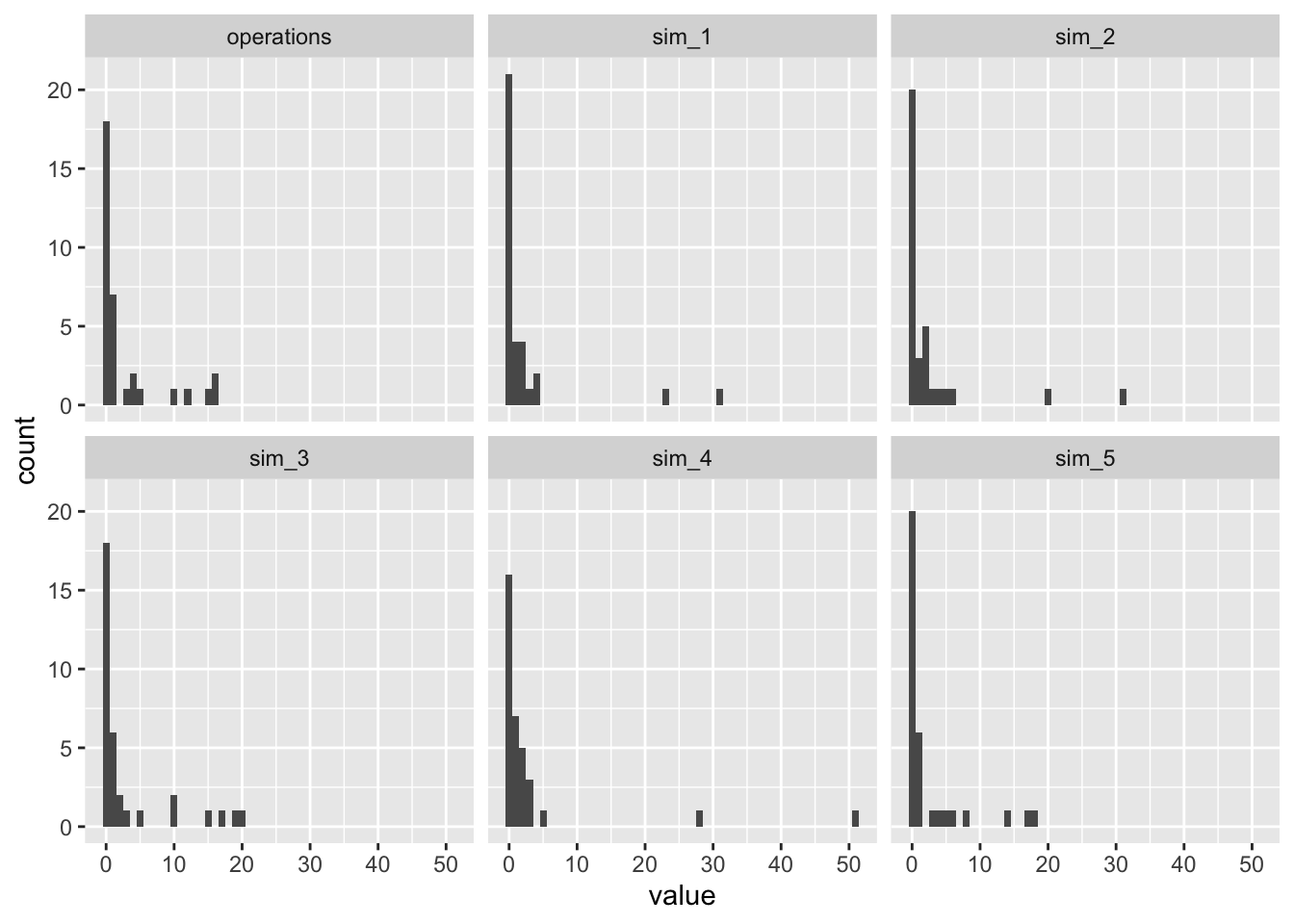
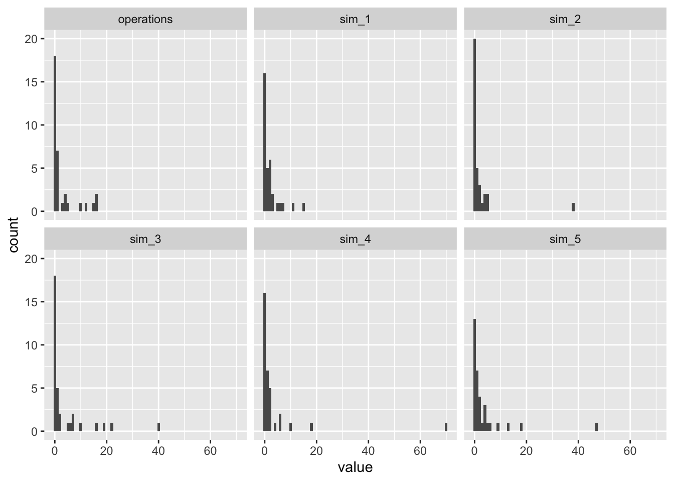
Notice that the negative binomial model as too many large values. I have a subtle intuition that the negative binomial is struggling to simultaneously capture the (1) mean, (2) the large spike at zero, and (3) the relative absence of large values.

To address this, we might add a component to the model to inflated the number of zeros relative to the usual negative binomial distribution.

It is fairly common for count data to have lots of zeros. We can imagine this substantively by thinking of two different processes. One process determines whether the observation is at risk of any events at all. Another process determines the number of events, which might still be zero.¹

¹ This “two process” motivation is simply a story to motivate the model—don’t take it too literally, especially when interpreting parameter estimates.

We can model as excess of zeros using a zero-inflation model. A zero-inflation model has two steps. In the first step, we have a logit model that determines whether the observation will equal zero or be a draw from some distribution.

15.1 Negative Binomial case

Let’s first consider zero-inflation in the negative binomial. How could we model an excess of zeros for an NB baseline distribution?

15.1.1 pmf

Let \(f(y_i; \mu_i, \theta)\) denote the pmf of a negative binomial distribution with mean \(\mu_i\) and dispersion \(\theta\).² We assume that observation \(i\) comes from

² This the nbinom2 parameterization with overdispersion parameter \(\theta\), where \(\text{Var}(Y_i) = \mu_i + \mu_i^2/\theta\)).

\[ y_i \sim \begin{cases} 0 & \text{with probability } \pi_i, \\ \text{NB}(\mu_i, \theta) & \text{with probability } 1 - \pi_i, \end{cases} \]

where \(\pi_i \in (0,1)\) is the probability of a structural zero. The remaining values follow the usual negative binomial distribution.³

³ Important note: even in an observation is not a structure zero, it still might equal zero, because the negative binomial has positive probability on zero as well. So there are two ways to get a zero.

Equivalently, the pmf of \(y_i\) can be written as

\[ f(y_i; \pi_i, \mu_i, \theta) = \begin{cases} \pi_i + (1 - \pi_i) f(0; \mu_i, \theta) & \text{if } y_i = 0 \\[6pt] (1 - \pi_i) f(y_i; \mu_i, \theta) & \text{if } y_i \neq 0 \end{cases}. \]

15.1.2 Likelihood

Create an indicator variable \(z_i = \mathbf{1}(y_i = 0)\) that equals one if \(y_i = 0\) and zero otherwise. Then for independent \(y_1, \dots, y_n\), the likelihood is

\[ L(\pi, \mu, \theta) = \prod_{i=1}^n \Bigg\{ \big[ \pi_i + (1 - \pi_i) f(0; \mu_i, \theta) \big]^{z_i} \cdot \big[ (1 - \pi_i) f(y_i; \mu_i, \theta) \big]^{1 - z_i} \Bigg\}. \]

15.1.3 Log-Likelihood

Taking logs, the log-likelihood is

\[ \ell(\pi, \mu, \theta) = \sum_{i=1}^n \Bigg\{ z_i \cdot \log\big( \pi_i + (1 - \pi_i) f(0; \mu_i, \theta) \big) + (1 - z_i) \cdot \big[ \log(1 - \pi_i) + \log f(y_i; \mu_i, \theta) \big] \Bigg\}. \]

We can imagine that \(\pi_i = \text{logit}^{-1}(Z\gamma)\) and \(\mu_i = \exp(X\beta)\), with \(\theta\) modeled as in a standard negative binomial regression.

15.1.4 In R

We can fit the zero-inflated negative binomial using the glmmTMB() function in R. Create the design matrix X with formula (for \(\mu_i = \exp (X\beta)\)) and the design matrix Z with ziformula (for \(\pi_i = \text{logit}^{-1} (Z\gamma)\)). The family nbinom2 specifies the negative binomial with variance \(\mu + \mu^2/\theta\) (which matrix MASS::glm.nb())

• glmmTMB() has a simulate() method to simulate from the predictive distribution.
• glmTMB() works well with {marginaleffects}.

15.1.4.1 Constant \(\pi\)

# formula
f <- operations ~ lower + vendors + budget + population

# zinb regression
library(glmmTMB)
zinb_fit <- glmmTMB(
  formula = f,  # usual nb part
  ziformula = ~ 1, # zero-inflation (logit) w/ intercept only
  family = nbinom2,  # "theta parameterization"
  data = sant
)

Then we can use simulate() to simulate from the predictive distribution and plot it in the usual way.

# simulate from predictive distribution
zinb_sims <- simulate(zinb_fit, nsim = 5)

# plot
bind_cols(sant, zinb_sims) |>
  pivot_longer(cols = c(operations, starts_with("sim_"))) |>
  separate(name, into = c("type", "sim_id"), sep = "_", remove = FALSE) |>
  ggplot(aes(x = value)) + 
  facet_wrap(vars(name)) +
  geom_histogram(center = 0, binwidth = 1)

15.1.4.2 \(\pi_i = \text{logit}^{-1}(X\beta)\)

# formulas
f <- operations ~ lower + vendors + budget + population
zi_f <-  ~ lower + vendors + budget + population

# zinb regression
zinb2_fit <- glmmTMB(
  formula = f,  
  ziformula = zi_f, # 🆕 model zi using covariates
  family = nbinom2,  
  data = sant
)

Then we can use simulate() to simulate from the predictive distribution and plot it in the usual way.

# simulate from predictive distribution
zinb2_sims <- simulate(zinb2_fit, nsim = 5)

# plot
bind_cols(sant, zinb2_sims) |>
  pivot_longer(cols = c(operations, starts_with("sim_"))) |>
  separate(name, into = c("type", "sim_id"), sep = "_", remove = FALSE) |>
  ggplot(aes(x = value)) + 
  facet_wrap(vars(name)) +
  geom_histogram(center = 0, binwidth = 1)

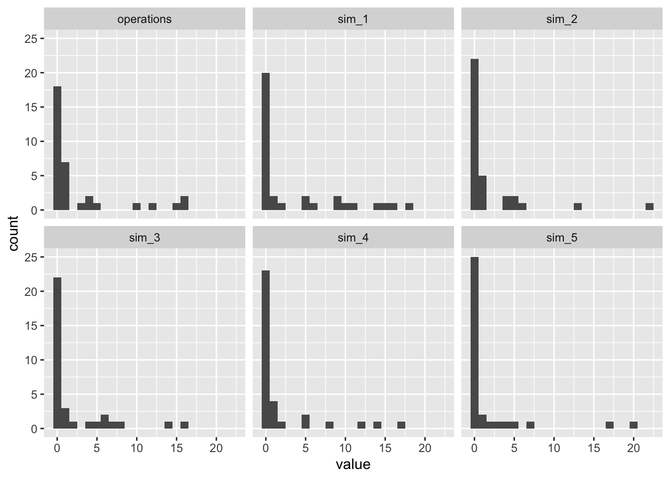
The predictive distributions for both ZINB models look much better. Because the zero-inflated part of the model handles the spike at zero, the negative binomial part of the model can better match the remainder of the distribution.

15.1.5 IC

The BIC likes the ZINB model with covariates best, and the model without zero-inflation is a close second.

BIC(nb_fit, zinb_fit, zinb2_fit) |>
  mutate(diff_min = BIC - min(BIC),
         post_prob = exp(-0.5*diff_min)/sum(exp(-0.5*diff_min)))

          df      BIC  diff_min  post_prob
nb_fit     6 142.8430 0.5379471 0.40320644
zinb_fit   7 146.3694 4.0643077 0.06914933
zinb2_fit 11 142.3051 0.0000000 0.52764423

The AIC likes the ZINB model with covariates best and the other two models aren’t particularly close.

AIC(nb_fit, zinb_fit, zinb2_fit) |>
  mutate(diff_min = AIC - min(AIC),
         akaike_weights = exp(-0.5*diff_min)/sum(exp(-0.5*diff_min)))

          df      AIC diff_min akaike_weights
nb_fit     6 133.6848  8.16975    0.016446724
zinb_fit   7 135.6848 10.16975    0.006050412
zinb2_fit 11 125.5151  0.00000    0.977502864

15.1.6 {marginaleffects}

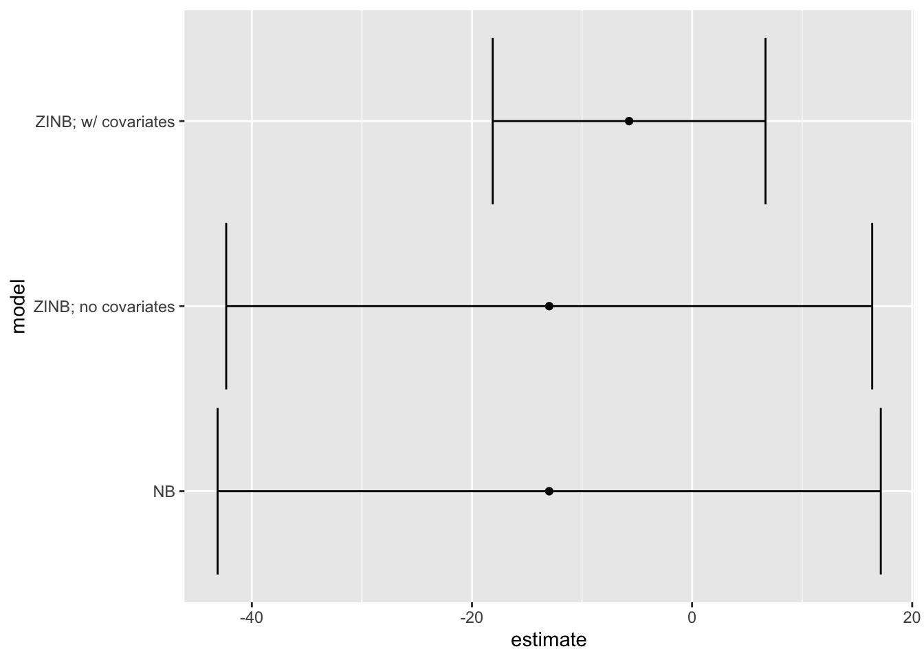
We can use the avg_comparisons() function to compute the average first difference as we move lower from its min to its max, averaging across the observed values of all the other covariates.

# compute avg. fd
avg_comparisons(nb_fit, variables = list(lower = "minmax"))

 Estimate Std. Error      z Pr(>|z|)   S 2.5 % 97.5 %
      -13       15.4 -0.845    0.398 1.3 -43.1   17.1

Term: lower
Type: response
Comparison: Max - Min

avg_comparisons(zinb_fit, variables = list(lower = "minmax"))

 Estimate Std. Error      z Pr(>|z|)   S 2.5 % 97.5 %
      -13         15 -0.867    0.386 1.4 -42.3   16.4

Term: lower
Type: response
Comparison: Max - Min

avg_comparisons(zinb2_fit, variables = list(lower = "minmax"))

 Estimate Std. Error      z Pr(>|z|)   S 2.5 % 97.5 %
    -5.72       6.32 -0.905    0.365 1.5 -18.1   6.67

Term: lower
Type: response
Comparison: Max - Min

# compute avg. fd
nb_fd <- avg_comparisons(nb_fit, variables = list(lower = "minmax"))
zinb_fd <- avg_comparisons(zinb_fit, variables = list(lower = "minmax"))
zinb2_fd <- avg_comparisons(zinb2_fit, variables = list(lower = "minmax"))

# plot
list("NB" = nb_fd, 
     "ZINB; no covariates" = zinb_fd,
     "ZINB; w/ covariates" = zinb2_fd) |>
  bind_rows(.id = "model") |>
  ggplot(aes(x = estimate, xmin = conf.low, xmax = conf.high,
             y = model)) + 
  geom_errorbarh() + 
  geom_point()

Warning

It’s worth pointing out that the sant dataset only has 34 observations and the zero-inflated negative binomial model with covariates has 11 parameters. This is small enough that we might worry about asymptotic approximations.

15.2 Poisson case

We could similarly use a zero-inflated Poisson. It follows the same logic. But it seems very usual in practice to have zero-inflation without over-dispersion, so I’ll just mention the possibility.

15.3 Other cases

We can easily extend this logic to other distributions as well. For example, we might imagine that some variables, like trade (in dollars) between two countries, might have a continuous distribution with a spike at zero. In this case, we could imagine a zero-inflated normal, for example.