Week 3 Exercises

Complete solutions open Friday, September 11 at 12:00 PM

These exercises practice the ideas in the week’s notes: the sampling distribution, the parametric bootstrap, the Fisher information matrix, the delta method, and evaluating confidence intervals. Read the notes first; the exercises assume them.

Do all the exercises below. The Extra Practice problems at the end are optional: they’re there if you want another repetition of a particular skill, and each one says which required exercise it pairs with.

Several exercises ask you to write down a prediction before running code. No one checks these predictions. You’ll just learn more if you commit to a guess before you peek.

If you jot down roughly how long each exercise took you, send it my way. I use it to size future sets, and right now I’m mostly guessing.

Sampling Distributions and the Bootstrap

Exercise 1 Defining the Sampling Distribution

In your own words, state what a sampling distribution is.
The notes give two uses for the sampling distribution. Name both.

For part (a)

The sampling distribution chapter states this definition explicitly, in one sentence, in the paragraph right before the heading “Example: The Toothpaste Cap Problem.” Find that sentence and put it in your own words, rather than reconstructing a definition from the simulation that follows it.

For part (b)

The sampling distribution chapter’s “Bias” section opens by asking how the sampling distribution actually gets used, then answers with a two-item numbered list. Read that list and name the two uses in your own words, not the notes’ phrasing.

Exercise 2 SD of the Bernoulli Estimator

For a Bernoulli sample of size $n$ with true parameter $\pi$, $\hat\pi = \operatorname{avg}(y)$.

Write the general formula for $\text{SD}(\hat\pi)$ — the SD of $\hat\pi$’s sampling distribution.
For $N = 150$ and $\pi = 0.05$, compute the number.

For part (a)

$\hat\pi = \operatorname{avg}(y)$ is the mean of $n$ independent Bernoulli($\pi$) draws. Turning $\text{Var}(y_i)$ into $\text{Var}(\hat\pi)$ takes two variance rules: one for summing independent variables, one for multiplying by a constant. The sampling distribution chapter applies both to this exact model, as its own worked example right after the definition of standard error. Open it and match its steps to your $y_i$.

For part (b), self-check

Once you have a number for part (b), check it by simulation instead of trusting the arithmetic alone. But supply your own value first, so the code can only tell you whether the two agree, not what either one is.

bsd_hint_my_answer <- NA # replace NA with your part (b) answer
abs(sd(replicate(10000, mean(rbinom(150, size = 1, prob = 0.05)))) - bsd_hint_my_answer) < 0.005

Fill in bsd_hint_my_answer and run it. TRUE means your value agrees with the simulation within Monte Carlo noise.

Exercise 3 Does the Odds Transform Preserve Unbiasedness?

$\hat\pi$ is unbiased for $\pi$: $E(\hat\pi) = \pi$. Is $\hat\pi/(1-\hat\pi)$ unbiased for the odds $\pi/(1-\pi)$? Answer in one sentence, and say why.

Hint

$E(a\hat\pi + b) = aE(\hat\pi) + b$ for constants $a$ and $b$: expectation distributes over addition and scalar multiplication. Does it distribute over division the same way? Write out $E\!\left(\hat\pi/(1-\hat\pi)\right)$ and try the same term-by-term move you’d use on $a\hat\pi + b$ to find out.

Self-check

The Bernoulli bias example under the notes’ “Bias” heading sets up exactly this transformation for the toothpaste-cap problem ($N = 150$, $\pi = 0.05$): it simulates $\hat\pi$ many times, forms $\hat\pi/(1-\hat\pi)$ on each draw, and compares the simulated average to the true odds $\pi/(1-\pi)$. Work through that comparison (on paper, or by running the chapter’s code) to check the conclusion you reached above.

Exercise 4 Bias versus Standard Error

The notes give bias and the standard error separate definitions, both properties of $\hat{\theta}$’s sampling distribution. State the difference in one sentence each:

What does it mean for $\hat{\theta}$ to be biased?
What does the standard error of $\hat{\theta}$ measure?

Hint

The notes give bias and the standard error their own sections, each with a labeled definition box: one under the Bias heading, one under the Standard Error heading. Reread the box for each term and write your own one-sentence version of it rather than quoting it directly: the exercise is checking that you can restate the idea, not that you can find it.

Self-check

Once you’ve drafted sentences for (a) and (b), try swapping them: read your (a) sentence as if it were answering (b), and vice versa. If either one still sounds like a reasonable description of the other property, it isn’t specific enough yet. Revise it so it only fits the definition it’s paraphrasing.

Exercise 5 Steps of the Parametric Bootstrap

In your own words, state the four steps of the parametric bootstrap algorithm from the notes’ chapter on the parametric bootstrap. Answer in one sentence per step.

What do you need before you start — the algorithm’s inputs?
What’s the first thing you compute, using just the observed data?
What happens once, for each of the $B$ replicates $b = 1, \dots, B$?
Once you have all $B$ replicate values, what do you do with them?

Hint

The chapter on the parametric bootstrap sets its steps off in a box labeled “Algorithm: Parametric Bootstrap Estimator,” right after the callout note comparing the parametric bootstrap to its nonparametric alternative. That box numbers on two levels: an outer list, and, inside one of its items, an inner list of the actions that happen together on a single pass. Match each part below to one outer item: the item that contains the inner list is still just one of them.

Self-check for part (c)

Self-check: once you’ve drafted your sentence for part (c), reread the first sub-item under the b-loop in the algorithm box (the one carrying a footnote) and compare it to what you wrote. If your sentence has the algorithm resampling the observed data points instead, that’s the nonparametric bootstrap. Revise your sentence to match what that sub-item says instead.

Fisher Information

Exercise 6 Observed Information to Standard Errors

Here is an observed information matrix for a two-parameter model, evaluated at $\hat\theta = (\hat\theta_1, \hat\theta_2)$:

\[ \mathcal{I}_{\text{obs}}(\hat\theta) = \begin{bmatrix} 5 & 1 \\ 1 & 2 \end{bmatrix} \]

By hand:

Find $\widehat{\text{SE}}(\hat\theta_1)$.
Find $\widehat{\text{SE}}(\hat\theta_2)$.

Hint 1

The Fisher information chapter’s section on more than two parameters writes out this same problem for a general $k \times k$ matrix. It shows exactly what gets inverted, and in what order, to reach $\widehat{\operatorname{Var}}(\hat\theta)$. Line up your $2\times2$ case against that pattern before doing any arithmetic on $\mathcal{I}_{\text{obs}}(\hat\theta)$.

Hint 2

The notes never spell out how to invert a $2\times2$ matrix by hand, so here is the rule: for $\begin{bmatrix} a & b \\ c & d \end{bmatrix}$, the inverse is $\dfrac{1}{ad-bc}\begin{bmatrix} d & -b \\ -c & a \end{bmatrix}$. In words: swap the two diagonal entries, negate the two off-diagonal entries, and divide the result by the determinant $ad-bc$. Apply that to $\mathcal{I}_{\text{obs}}(\hat\theta)$ to get $\widehat{\operatorname{Var}}(\hat\theta)$.

Exercise 7 Hessian to Covariance Matrix

You’ve fit a model with optim(par, fn, control = list(fnscale = -1), hessian = TRUE), where fn returns the log-likelihood $\ell(\theta)$, not its negative, and the result is stored in est. Write the one line of R that turns est$hessian into $\widehat{\operatorname{Var}}(\hat\theta)$, the estimated covariance matrix of $\hat\theta$.

Hint

You already know from the call in the prompt that fn computes $\ell(\theta)$ directly, not $-\ell(\theta)$: fnscale = -1 only tells optim() how to treat that value internally while it searches. The beta-model walkthrough in the Fisher information chapter builds a call structured exactly like yours, optim(..., control = list(fnscale = -1), hessian = TRUE), and the numbered comment on that hessian = TRUE line settles what the returned hessian is a Hessian of. Reread that comment before you decide what has to happen to est$hessian on the way to a covariance matrix.

Self-check

A covariance matrix cannot have negative diagonal entries. Fit any model with optim(..., hessian = TRUE), apply your candidate line, and check diag() of the result: non-negative entries confirm the sign is resolved, a negative entry means it isn’t.

Exercise 8 The Wald Interval Formula

Write the general formula for a Wald confidence interval on a scalar parameter $\hat\theta$ estimated by maximum likelihood.

The 90% interval.
The 95% interval.

Hint

The Fisher information chapter has a section right after it finishes the general variance-matrix formula for several parameters (titled “From Curvature to Wald Confidence Intervals”) that works out this exact interval: a scalar parameter estimated by maximum likelihood, at 90% and 95%. Open that section and adapt what’s there to your own notation.

Self-check

Once you’ve written both intervals, check your critical values independently of the notes: a two-sided interval splits its leftover probability evenly between the two tails, so the tail probability you hand to R’s qnorm() isn’t your confidence level itself.

# tail probability = 1 - (1 - confidence level) / 2
qnorm(0.95)    # should match your critical value for part (a)
qnorm(0.975)   # should match your critical value for part (b)

The Delta Method

Exercise 9 The Delta-Method Variance Formula

In the one-parameter case, write the delta-method approximation for $\widehat{\operatorname{Var}}[\tau(\hat\theta)]$ in terms of $\tau'(\hat\theta)$ and $\widehat{\operatorname{Var}}(\hat\theta)$.

Hint

The chapter builds this exact one-parameter result from a first-order Taylor expansion of $\tau$ around $\hat\theta$, in the discussion right before the worked examples that follow (the Bernoulli odds, the Poisson SD, and the beta mean). Which classic rule for the variance of a linear transformation does that expansion invoke? Reread that discussion and use the rule it names to fix the form of your answer.

Self-check

A variance can never be negative, no matter the sign of $\tau'(\hat\theta)$. Plenty of transformations $\tau$ are decreasing, which makes $\tau'(\hat\theta)$ negative. Take your candidate formula and ask whether it could go negative for such a $\tau$, given that $\widehat{\operatorname{Var}}(\hat\theta)$ itself is never negative. A linear (unsquared) power on $\tau'(\hat\theta)$ can flip the sign of the whole expression, so any candidate built that way cannot be right.

Exercise 10 Gradient of a Ratio

Let $\tau(a, b) = \dfrac{a}{a+b}$ — the same ratio form as the beta mean in the notes, but with generic $a$ and $b$ in place of $\alpha$ and $\beta$.

Find $\dfrac{\partial \tau}{\partial a}$ and $\dfrac{\partial \tau}{\partial b}$.
Assemble your two partials into the gradient $\nabla \tau(a, b)$.

Hint

The delta-method chapter uses $\nabla\tau(\hat\theta)$ throughout but never restates the calculus rule for differentiating a ratio, so it’s worth having on hand: for $\tau = u/v$, $\dfrac{\partial \tau}{\partial x} = \dfrac{u'v - uv'}{v^2}$, where $u'$ and $v'$ are the derivatives of $u$ and $v$ with respect to $x$. Set $u = a$ and $v = a+b$, then apply the rule twice: once differentiating with respect to $a$ with $b$ held fixed, once differentiating with respect to $b$ with $a$ held fixed.

Self-check

Once you have both partials, check them numerically rather than eyeballing the signs. numDeriv::grad() (the delta-method chapter’s own numerical-gradient section uses it the same way) nudges each argument of a function and reports how the output moves, giving you a numerical gradient to compare against your analytic one.

gr_hint_tau <- function(theta) {
  a <- theta[1]
  b <- theta[2]
  a / (a + b)
}

gr_hint_point <- c(a = 3, b = 7)

numDeriv::grad(gr_hint_tau, gr_hint_point)

# now evaluate your own d/da and d/db formulas at gr_hint_point and compare

Bias and Precision

Exercise 11 Average versus Median

Suppose you plan to sample $N$ observations from a normal distribution and use the sample to estimate the center of the distribution. You are choosing between two estimators: the sample average $\operatorname{avg}(y)$ and the sample median. Before you run anything, predict which of the two has the smaller SE, and explain why using a mechanism — not a guess, and not “because a simulation shows it.”
Check your prediction with a Monte Carlo simulation. Choose a sample size $N$, a mean $\mu$, and an SD $\sigma$; choose a number of simulated samples, and set a seed. For each simulated sample of size $N$ drawn from a normal($\mu$, $\sigma$) distribution, compute $\operatorname{avg}(y)$ and the median. Treat the SD of the resulting averages across simulations as a Monte Carlo estimate of the SE of $\operatorname{avg}(y)$, and do the same for the median. Report both estimated SEs and their ratio. Does the ratio match your prediction in (a)?

For part (a)

The notes define the SE as simply the standard deviation of the sampling distribution, and the normal-model example works out $\text{Var}[\operatorname{avg}(y)] = \sigma^2/N$ because $\operatorname{avg}(y)$ can be written as the explicit sum $\frac{1}{N}\sum_{i=1}^N y_i$, to which the variance-of-independent-sum rule applies term by term. Can you write the sample median as that same kind of explicit weighted sum of $y_1, \dots, y_N$? Write both estimators as explicit formulas in the data before you commit to a prediction, and build your explanation from that comparison.

For part (b), self-check

The sampling-distribution chapter’s Standard Error section already runs this exact workflow in its “Example: Exponential Model”: loop over many simulated samples, recompute the estimator on each one, and take the SD of the resulting vector as the simulated SE. It does this for a case where the SE has no clean closed form. Adapt that loop by drawing from rnorm() and computing both mean() and median() inside each iteration. Once you have a simulated SE for $\operatorname{avg}(y)$, compare it to $\sigma/\sqrt{N}$ using the $\mu$, $\sigma$, and $N$ you chose, since the notes show this is the exact SE of $\operatorname{avg}(y)$ for a normal model. A mismatch there means a bug to chase down before you trust the ratio.

Exercise 12 One Unbiased, One Biased

Let $X_1, \dots, X_N$ be an iid sample from an exponential distribution with rate $\lambda$, so $E(X) = 1/\lambda$. Define the population mean $\mu = 1/\lambda$, estimated by $\hat\mu = \operatorname{avg}(x)$, and recall from Week 2’s exercise “The Exponential Model” that the ML estimate of the rate is $\hat\lambda = 1/\operatorname{avg}(x)$.

Show that $\hat\mu = \operatorname{avg}(x)$ is unbiased for $\mu$.
Show that $\hat\lambda = 1/\operatorname{avg}(x)$ is biased for $\lambda$, and say whether it over- or underestimates $\lambda$ on average.

For part (a)

The notes’ definition of bias says $\hat\theta$ is unbiased exactly when $E(\hat\theta) = \theta$, not merely close to it. Write $\operatorname{avg}(x)$ as $\frac{1}{N}\sum_{i=1}^N X_i$, take the expectation of that sum directly, and use the fact that expectation is linear and every $X_i$ shares the same expectation as $X$.

For part (b)

Part (a)’s trick relied on $g(t) = t$ being linear, so the expectation passed straight through the sum. $g(t) = 1/t$ is not linear, so that trick does not carry over to $\hat\lambda = 1/\operatorname{avg}(x)$. Check whether $g(t) = 1/t$ is convex or concave for $t > 0$ by computing its second derivative, which determines which way Jensen’s inequality runs: for a convex $g$, $g(E[T]) \leq E[g(T)]$, and for a concave $g$ the inequality reverses. Apply whichever branch matches your check, with $T = \operatorname{avg}(x)$.

Standard Errors in Practice

Exercise 13 The Poisson Standard Error

Suppose $y_1, \dots, y_N$ are an iid sample from a Poisson model, $f(y_i \mid \lambda) = \dfrac{\lambda^{y_i} e^{-\lambda}}{y_i!}$ for $y_i = 0, 1, 2, \dots$. Derive $\widehat{\text{SE}}(\hat\lambda)$ from the observed Fisher information, using the same steps as the exponential example in the notes.

Write the log-likelihood $\ell(\lambda)$ for the sample and find the score function $\partial \ell(\lambda)/\partial \lambda$.
Find the second derivative $\partial^2 \ell(\lambda)/\partial \lambda^2$, and set the score to zero to solve for $\hat\lambda$.
Evaluate the second derivative at $\hat\lambda$ to get the observed information $\mathcal I_{\text{obs}}(\hat\lambda)$, invert it, and take the square root to get $\widehat{\text{SE}}(\hat\lambda)$.

For part (a)

Two familiar log rules (the power rule and the product rule for logarithms) turn the product inside the Poisson pmf into a sum you can differentiate term by term. Apply both to $\log\!\left(\lambda^{y_i}e^{-\lambda}/y_i!\right)$ before summing over $i$. One of the resulting three terms will not involve $\lambda$ at all.

For part (c)

Part (b) already gives you $\sum_{i=1}^N y_i$ written in terms of $N$ and $\hat\lambda$. Substitute that expression into the second derivative before evaluating at $\hat\lambda$, rather than evaluating with the raw sum still sitting in the formula.

Exercise 14 The Bogotá Operations Mismatch

In Week 2’s exercise “The SD the Model Implies,” you compared the Poisson model’s predictive SD to the sample SD for several cities’ enforcement-operations counts, and Bogotá’s numbers didn’t match. Here you work through Bogotá on its own, add a standard error, and pin down exactly what the mismatch is telling you.

op_holland2015 <- crdata::holland2015
op_ops <- op_holland2015$operations[op_holland2015$city == "bogota"]

op_ops holds the 19 district-level operations counts for Bogotá.

Find the ML estimate $\hat\lambda$ of the Poisson rate, and its standard error $\widehat{\text{SE}}(\hat\lambda)$, using the result you derived in Exercise 13.
Find the standard deviation the Poisson model implies for individual operations counts, and compare it to the sample SD of op_ops.
Using the ratio of the sample variance to the sample mean, diagnose the mismatch: which structural assumption of the Poisson model do these data violate, and why can’t a single parameter $\hat\lambda$ satisfy both quantities at once?

For part (b)

By the time you reach (b), you already have a number from (a): the standard error of $\hat\lambda$, which measures how much the estimate would move if you redrew the sample of 19 districts. Is that the same thing as how spread out individual operations counts are under the model? The delta-method chapter’s “Poisson: From $\lambda$ to SD” section gives the population standard deviation of a Poisson variable in one line. Use $\hat\lambda$ in place of $\lambda$ there to get the quantity part (b) is asking for.

Self-check for part (c)

If a Poisson model with your $\hat\lambda$ were exactly right for these data, the ratio of sample variance to sample mean should behave like a ratio computed from genuine Poisson draws of the same size: it should cluster near 1, with some sampling noise for $N = 19$. Simulate many samples of that size from a Poisson($\hat\lambda$), compute the same ratio for each, and see where Bogotá’s actual ratio falls relative to that simulated spread.

# simulate many samples of size N from Poisson(lambda_hat) and see where
# the real var/mean ratio falls among the simulated ratios
op_hint_lambda_hat <- mean(op_ops)
op_hint_n <- length(op_ops)
op_hint_n_sims <- 2000
op_hint_ratios <- numeric(op_hint_n_sims)
for (i in 1:op_hint_n_sims) {
  op_hint_y <- rpois(op_hint_n, op_hint_lambda_hat)
  op_hint_ratios[i] <- var(op_hint_y) / mean(op_hint_y)
}
range(op_hint_ratios)

Exercise 15 Exponential SE via the Delta Method

Return to the exponential model, $f(y_i \mid \lambda) = \lambda \exp(-\lambda y_i)$ for $y_i \ge 0$ and $i = 1, \dots, N$. Week 2’s “The Exponential Model” found the ML estimate $\hat\lambda = 1/\operatorname{avg}(y)$.

Derive $\widehat{\text{SE}}(\hat\lambda)$ from the observed Fisher information.
The mean of the exponential distribution is $\mu = 1/\lambda$. Use the delta method to derive $\widehat{\text{SE}}(\hat\mu)$, and simplify your answer as far as it goes.

For part (a)

The Fisher information chapter’s “Approximations via asymptotics” callout is followed immediately by the general recipe for turning the curvature of a log-likelihood into a standard error, the same recipe you built in Exercise 6. Differentiate the log-likelihood given above twice, then apply that recipe to your own second derivative.

For part (b)

The delta method chapter states the general one-parameter formula before any of its worked examples (the same formula behind Exercise 9), and its Poisson-to-SD example carries out the same differentiate-then-square maneuver for a different transformation of a rate parameter. Find $\tau'(\lambda)$ for $\tau(\lambda) = 1/\lambda$, then combine it with your part (a) variance in that formula.

Self-check

The delta method chapter verifies its Poisson-to-SD result the same way: simulate many data sets from a known rate, recompute the estimate on each one, and compare the spread of those estimates to the closed-form SE. Do the same here for both $\hat\lambda$ and $\hat\mu$, and confirm your two formulas track the simulated spread.

# self-check: simulated SE vs. your closed-form formulas
exp_se_delta_n <- 200
exp_se_delta_lambda_true <- 3
exp_se_delta_n_sim <- 10000

exp_se_delta_lambda_hats <- numeric(exp_se_delta_n_sim)
exp_se_delta_mu_hats <- numeric(exp_se_delta_n_sim)

for (exp_se_delta_s in 1:exp_se_delta_n_sim) {
  exp_se_delta_y <- rexp(exp_se_delta_n, exp_se_delta_lambda_true)
  exp_se_delta_lambda_hats[exp_se_delta_s] <- 1 / mean(exp_se_delta_y)
  exp_se_delta_mu_hats[exp_se_delta_s] <- mean(exp_se_delta_y)
}

sd(exp_se_delta_lambda_hats)  # compare to your part (a) formula, evaluated near lambda_true
sd(exp_se_delta_mu_hats)      # compare to your part (b) formula, evaluated near 1 / lambda_true

Exercise 16 SE of a Ratio by Hand

Take the fitted values and covariance matrix from the notes’ beta-model example: $\hat\theta = (\hat a, \hat b) = (37.08, 114.93)$ and

\[ \widehat{\operatorname{Var}}(\hat\theta) = \begin{bmatrix} 5.96 & 18.41 \\ 18.41 & 57.84 \end{bmatrix}. \]

Here the quantity of interest is not the notes’ $\mu = a/(a+b)$ but the ratio $\tau = a/b$, so relabel the fitted values $\hat a$ and $\hat b$ rather than $\hat\alpha$ and $\hat\beta$.

Write $\nabla\tau(\theta)$ and evaluate it at $\hat\theta$.
Compute $\widehat{\operatorname{Var}}(\hat\tau)$ by hand. Write out each of the four products in the sum, and identify the two that come from the off-diagonal entries of $\widehat{\operatorname{Var}}(\hat\theta)$.
Compute $\widehat{\text{SE}}(\hat\tau)$ from your answer to (b).
Confirm (b) and (c) in R.

Hint

The fitted values and covariance matrix here are lifted from the notes’ beta-model example, but that chapter’s delta-method derivation is for a different $\tau$. Two of its subsections carry out the same two moves you need: “The gradient” gives $\partial\mu/\partial\alpha$ and $\partial\mu/\partial\beta$ for $\mu = \alpha/(\alpha+\beta)$ without showing the derivation — apply the quotient rule yourself to get there — and “By hand” (under “The matrix algebra”) expands the resulting sandwich product term by term. Use their algebraic layout as a template, substituting $\tau = a/b$ for $\mu = \alpha/(\alpha+\beta)$.

For parts (b) and (c)

Because $\widehat{\operatorname{Var}}(\hat\theta)$ has a sizable off-diagonal entry and the gradient’s two components have opposite signs, the terms in this sum partially cancel, leaving a result much smaller in magnitude than any one of them. Carry at least three or four significant figures through the gradient and every product, rounding only at the very end. Rounding early can shift your final variance and SE by a double-digit percentage.

Self-check

Once you have computed (b)-(c) by hand and confirmed them in R for part (d), the two should agree to two or three significant figures. If they don’t, check first whether you rounded the gradient or an intermediate product too early before you suspect your R code.

Exercise 17 The 2024 Turnout Bootstrap

State-level turnout among the voting-eligible population in the 2024 general election — one proportion per state, plus DC, 51 observations in all — is posted as a tibble in this gist (source: the UF Election Lab). Read it in and treat the 51 turnout proportions as a sample from a beta distribution.

a. Fit the beta distribution by maximum likelihood, the way the notes do for the beta example: write the log-likelihood and hand it to optim(). Report $\hat\alpha$ and $\hat\beta$, along with the implied mean $\hat\mu = \hat\alpha / (\hat\alpha + \hat\beta)$ and standard deviation $\hat\sigma = \sqrt{\hat\alpha\hat\beta \big/ \big((\hat\alpha+\hat\beta)^2(\hat\alpha+\hat\beta+1)\big)}$.

b. Get a parametric-bootstrap standard error for $\hat\mu$ and for $\hat\sigma$, using $B = 2000$ replicates — the same $B$ the notes use.

c. Some of your $B$ replicate fits will fail to converge. How many do, and what do you do about it?

For part (a)

“The beta example” names two things in this week’s chapters. The parametric bootstrap chapter fits a beta model by maximum likelihood as a warm-up before bootstrapping it. The Fisher information chapter fits a different beta model (Lahman batting averages) to get a Hessian-based covariance matrix instead: a different SE method entirely. Work from the parametric bootstrap chapter’s version: its log-likelihood function and optim() call carry over to tb_turnout$vep_turnout with only the data changed.

For part (b)

The parametric bootstrap chapter’s beta example already bootstraps a derived quantity rather than $\hat\alpha$ and $\hat\beta$ themselves: its last code block computes the mean from each refit’s shape parameters before taking the sd() of that column. $\hat\sigma$ is a second derived quantity of the same kind: apply the formula from part (a) to each replicate’s fit instead of deriving a new one.

For part (c)

optim()’s return value always carries a $convergence element. The Fisher information chapter’s beta-model function checks exactly this element and prints a warning whenever it is nonzero. Your part (b) loop already calls optim() on every replicate, so nothing needs refitting: pull that element off each replicate’s fit as you go and use it to find which ones failed.

Putting It Together

Exercise 18 Two Intervals at a Rare-Event Boundary

You observe $N = 20$ independent Bernoulli trials and exactly one success.

Construct the 95% Wald confidence interval for $\pi$ from this sample. What do you notice about where the interval falls?
Instead, construct a 95% confidence interval by parametric bootstrap: draw $B = 2{,}000$ bootstrap samples of size $N = 20$ from a Bernoulli($\hat\pi$) distribution, recompute $\hat\pi^*$ for each, and take the 2.5th and 97.5th percentiles of the $\hat\pi^*$ values. Compare where this interval falls to your answer in (a).
Now check both interval methods by simulation, at two settings: $\pi = .05, N = 20$ and $\pi = .10, N = 40$. For each setting, simulate a large number of studies — in each, draw a sample of size $N$ from Bernoulli($\pi$) and construct both intervals as in (a) and (b) — and report, for each interval method, the fraction of simulated studies that capture the true $\pi$. Also report, at each setting, the frequency with which $\hat\pi = 0$. Compare the two coverage rates to the nominal 95% rate and to each other, and explain why an interval that always stays inside $[0, 1]$ does not necessarily cover $\pi$ at the nominal rate.

For part (c): the nested loops

The natural approach to part (c) pastes together the notes’ coverage-simulation loop (the Evaluating Confidence Intervals chapter) and the notes’ parametric-bootstrap loop (the Parametric Bootstrap chapter). As written in each chapter, both loops count their iterations with the same variable, i. Nesting the bootstrap loop inside the coverage loop without renaming one of those counters means the inner loop finishes each pass with i sitting at its own last value, so the outer loop’s use of i to store that iteration’s result no longer tracks which outer iteration you’re on. Give the inner loop’s counter a name distinct from the outer loop’s before you nest it.

For part (c): checking capture

The notes’ own coverage-simulation example (the Evaluating Confidence Intervals chapter) checks capture with strict inequalities: the lower bound compared with < and the upper bound compared with > against the known true value. That’s fine there because the quantity being intervalled is continuous, so a computed bound landing exactly on the true value is a negligible possibility. Here, $\pi$ itself lies on the grid of values $\hat\pi$ can take, so a bound landing exactly on $\pi$ is a real, checkable event for either interval method, not a coincidence to ignore. Check capture with closed inequalities (<= on both sides), so a bound that lands exactly on $\pi$ counts as capturing it.

Exercise 19 Comparing Models of Coalition Duration

Cabinet coalitions in parliamentary democracies eventually break apart. The coalition data set in the brglm2 package records how long each of $N = 314$ coalition governments lasted, in months, alongside several covariates; you’ll use only the duration.

library(brglm2)
data("coalition", package = "brglm2")
dc_y <- coalition$duration

Some background. When you model duration data, it helps to think in terms of the hazard: the instantaneous risk of a coalition ending at time $t$, given that it has survived to $t$.

The exponential is the simplest choice. Its density is $f(t \mid \lambda) = \lambda e^{-\lambda t}$ for $t > 0$, its mean is $\mathbb{E}[T] = 1/\lambda$, and its hazard is the constant $h(t) = \lambda$: the risk of ending doesn’t depend on how long the coalition has already lasted.

The Weibull generalizes the exponential by letting the hazard rise or fall with time; setting its shape parameter $k = 1$ recovers the exponential exactly, while $k > 1$ gives a rising hazard and $k < 1$ a falling one. Its mean is $\mathbb{E}[T] = \lambda\,\Gamma(1 + 1/k)$.

The log-normal instead assumes $\log T \sim \mathcal{N}(\mu, \sigma^2)$. Its density is $f(t \mid \mu, \sigma) = \dfrac{1}{t\sigma\sqrt{2\pi}}\exp\!\left(-\dfrac{(\log t - \mu)^2}{2\sigma^2}\right)$ for $t > 0$, its mean is $\mathbb{E}[T] = \exp(\mu + \sigma^2/2)$, and its hazard rises and then falls.

You’ll fit the exponential and log-normal models by hand. Someone has already fit the Weibull for you and printed the result below — read it, don’t refit it.

Weibull fit (ML):
  k-hat (shape)      1.138   SE 0.052   95% CI [1.037, 1.240]
  lambda-hat (scale) 19.29
  mean duration      18.410  SE 0.914
  maximized log-lik  -1225.3
  AIC                2454.6

Part 1. Fit the exponential and log-normal models.

Write the exponential log-likelihood $\ell(\lambda)$ for dc_y, and maximize it with optim(), requesting the Hessian. Report $\hat\lambda$, its SE (invert the observed information, then take the square root), the maximized log-likelihood, and the AIC, where $\text{AIC} = 2p - 2\,\ell(\hat\theta)$ and $p$ is the number of parameters (smaller is better).
The exponential’s mean is $\tau(\lambda) = 1/\lambda$. Using the invariance property and the delta method, get the ML estimate of the mean duration and its SE.
Write the log-normal log-likelihood $\ell(\mu, \sigma)$ for dc_y (use dlnorm(dc_y, meanlog = mu, sdlog = sigma, log = TRUE)), and maximize it with optim() over $(\mu, \sigma)$, requesting the Hessian. Report $\hat\mu$, $\hat\sigma$, their covariance matrix, the maximized log-likelihood, and the AIC.
The log-normal’s mean is $\tau(\mu, \sigma) = \exp(\mu + \sigma^2/2)$. Using the invariance property and the multi-parameter delta method, get the ML estimate of the mean duration and its SE.

Part 2. The classical estimate.

Using dc_y directly, with no distributional assumption, compute $\operatorname{avg}(y)$ and its SE.

Part 3.

Collect all four estimates of the mean duration (classical, exponential, Weibull, log-normal), each with its SE, and the AIC of the three fitted models, in one table.
Which model does the AIC prefer? Which model’s estimate of the mean differs most from the other three? Are these the same model?
What does that combination tell you about how much the fit statistics can help you decide which estimate of the mean to trust?

For parts (a) and (c): the optim() + Hessian pattern

The notes’ Fisher-information chapter fits a model this same way, using the beta model and batting-average data: a log-likelihood function built from the distribution’s d*(..., log = TRUE) values and a parameter vector theta, one call to optim() with hessian = TRUE, then a covariance matrix from inverting the observed information. Part (a)’s exponential is the one-parameter version of that recipe; part (c)’s log-normal is the two-parameter version. Read the “Beta model and optim()” section for the full pattern, including how theta[1] and theta[2] pull the two parameters out of the vector optim() optimizes over.

For part (d): the multi-parameter delta method

Part (d) needs the two-parameter version of the same delta-method formula you used in part (b), now applied to a gradient with two entries instead of one. The notes’ delta-method chapter builds exactly this in the Beta Example section for the beta model’s mean. See “The gradient” and “The matrix algebra” for how the general formula turns into R code once you have the gradient vector. Differentiate $\tau(\mu,\sigma) = \exp(\mu + \sigma^2/2)$ with respect to $\mu$ and then with respect to $\sigma$ to get the two entries of that vector.

Self-check for parts (a), (b), and (e)

The notes’ exponential example notes that this model’s ML estimate has a closed form, $\hat\lambda = 1/\operatorname{avg}(y)$: optim() in part (a) should converge to the same value you’d get from that one-line formula. That closed form also means part (b)’s mean estimate, $1/\hat\lambda$, and part (e)’s classical mean, $\operatorname{avg}(y)$, are two routes to the same number: they should agree to several decimal places. If they don’t, tighten optim()’s convergence tolerance or check your starting value in (a) before moving to (c) and (d).

Exercise 20 German Tank Problem

Week 2’s exercise “The Discrete Uniform” derived two estimators for a discrete uniform model and closed by noting that an estimator’s weaknesses aren’t visible from its formula alone — you find them by asking how the estimator behaves under repeated sampling. This exercise asks that question directly.

Suppose $y_1, \dots, y_N$ are drawn independently from a discrete uniform distribution on $\{0, 1, \dots, K\}$, with pmf \[f(y; K) = \frac{1}{K+1}, \quad y \in \{0, 1, \dots, K\}.\] The maximum-likelihood estimator is $\hat K_{ML} = \max(y)$, and the method-of-moments estimator is $\hat K_{MM} = 2 \cdot \operatorname{avg}(y)$.

Note: this model violates several of the usual regularity conditions, so the standard asymptotic guarantees for ML estimators do not apply here.

Choose a value of $K$, and run a Monte Carlo simulation to find the bias and the variance of $\hat K_{ML}$ and of $\hat K_{MM}$ at a small ($N = 3$), a medium ($N = 25$), and a large ($N = 1000$) sample size.
In a single sentence, propose and defend a criterion for choosing between an estimator that is biased and one that is noisier but less biased, when you can report only one number.
Compute your criterion for both estimators at all three sample sizes.
State your recommendation.

For part (a)

The notes’ sampling-distribution chapter builds its Toothpaste Cap Problem sampling distribution the same way you’ll want to build yours here: a numeric container sized to the number of Monte Carlo replicates, and a for loop that draws one new data set per iteration and stores one number from it before moving to the next iteration. Set up that container-and-loop shell for the discrete uniform model described in this exercise, then run the whole thing separately for each of the three sample sizes named in the prompt.

For part (a), the code

Inside that loop, one call to sample() draws a single data set from the discrete uniform on $\{0, 1, \dots, K\}$ described in the prompt. From that one drawn data set you can compute both $\max(y)$ and $2 \cdot \operatorname{avg}(y)$ before the loop moves to its next iteration. A skeleton:

gt_K <- NA        # fill in: your chosen K
gt_N <- NA        # fill in: the sample size for this run
gt_n_sims <- NA   # fill in: number of Monte Carlo replicates

gt_ml_est <- numeric(gt_n_sims)  # container for hat K_ML
gt_mm_est <- numeric(gt_n_sims)  # container for hat K_MM

for (i in 1:gt_n_sims) {
  gt_y <- sample(0:gt_K, size = gt_N, replace = TRUE)
  gt_ml_est[i] <- max(gt_y)
  gt_mm_est[i] <- 2 * mean(gt_y)
}

Extra Practice

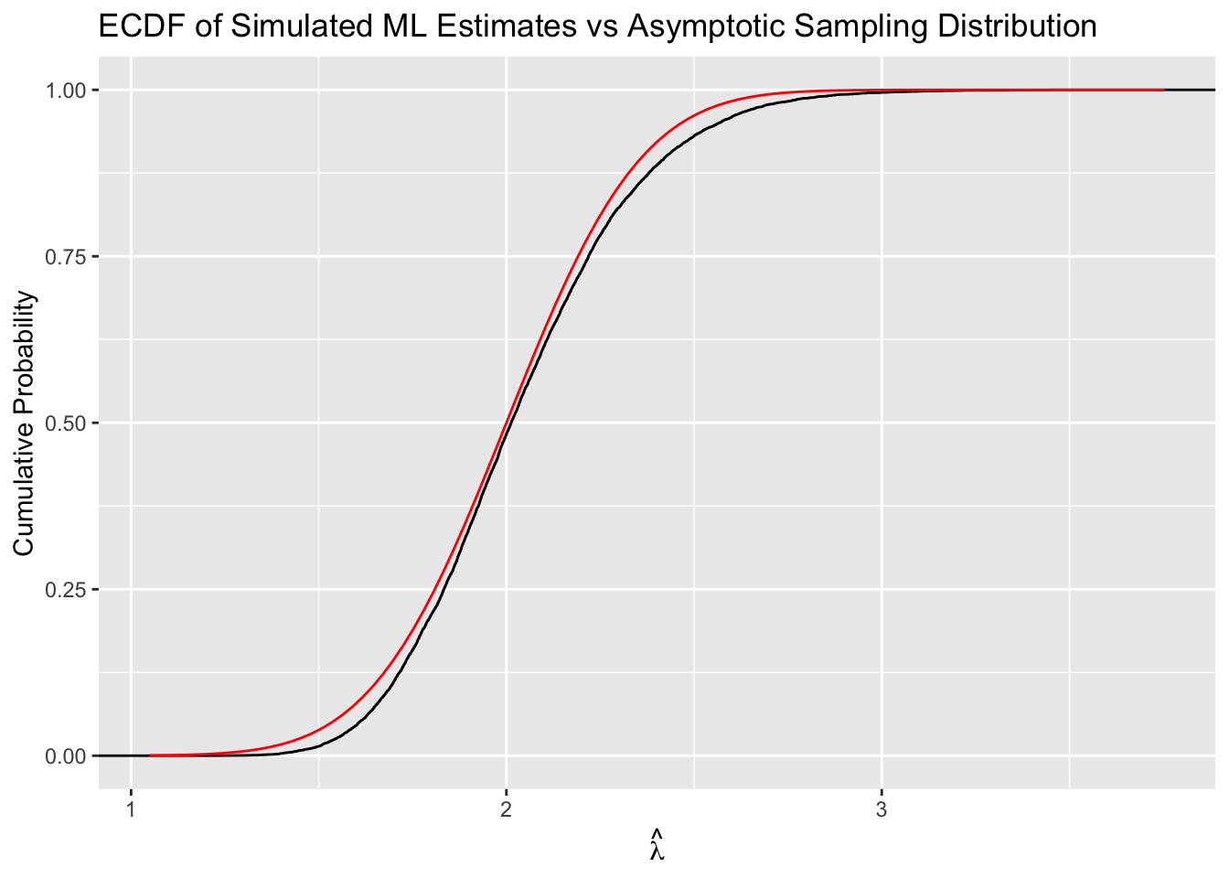
Extra Practice 1 Checking the Asymptotic Normal by Simulation

This item pairs with Exercise 15 and repeats its use of the asymptotic-normality and asymptotic-variance theorems, but this time you check the theorem’s prediction against a simulated sampling distribution instead of deriving $\widehat{\text{SE}}(\hat\lambda)$ from the log-likelihood.

Fix $\lambda = 2$ and $N = 50$ for an exponential model.

Simulate the sampling distribution of $\hat\lambda = 1/\operatorname{avg}(y)$: draw a large number of samples of $N$ observations from $\text{Exponential}(\lambda)$, compute $\hat\lambda$ for each sample, and report the simulated mean and SD of $\hat\lambda$ across samples.
Use the notes’ asymptotic normality theorem and asymptotic variance theorem to write down the normal distribution that $\hat\lambda$ should follow, in terms of $\lambda$ and $N$. Compare its mean and SD to what you found in part a.
Compare the shape of the simulated distribution to this asymptotic normal — for example, overlay the normal density on a histogram of your simulated $\hat\lambda$ values. (A quantile table or an ECDF overlay are optional further comparisons.) Where, if anywhere, does the simulated distribution depart from the normal approximation?

For part (a)

The sampling-distribution chapter’s toothpaste cap example builds a sampling distribution with the same shape this part needs: a container vector and a for loop that draws one sample, computes one estimate from it, and stores the estimate, repeated many times. Adapt that loop to draw one exponential sample of size $N$ per iteration and store $\hat\lambda$ in place of the toothpaste cap’s estimate. Before trusting the mean and SD that come out, check the Arguments section of ?rexp for what its rate argument means. Get that backward, and every number downstream describes a different $\lambda$ than the one you fixed.

For part (b)

You already derived the Fisher information for this exact exponential model when you worked Exercise 15. Reuse that calculus instead of redoing it from the log-likelihood. The piece you still need (how to turn Fisher information into the variance of $\hat\lambda$) is the notes’ asymptotic variance theorem, in the Fisher information chapter immediately after the asymptotic normality theorem.

For part (c)

The sampling-distribution chapter’s toothpaste cap example overlays a normal density on a histogram of simulated estimates using the same geom_histogram() / stat_function(fun = dnorm, ...) combination this part needs, but that example centers its curve on the simulated mean and SD. Here you want the curve centered on the asymptotic mean and SD from part b instead. Build your plot the same way, with that one substitution.

Extra Practice 2 SD of a Fitted Beta Model

This repeats Exercise 16’s delta-method skill — turning a covariance matrix for two fitted parameters into an SE for a function of them — but here you fit the model yourself, the function is the beta distribution’s SD rather than a ratio of its two parameters, and its gradient doesn’t simplify by hand, so you get it numerically.

Fit the beta model to Lahman’s 2023 batting averages, exactly as the notes do: battingStats(), yearID == 2023, AB >= 100, and optim() with hessian = TRUE to get $\hat\theta = (\hat\alpha, \hat\beta)$ and $\widehat{\operatorname{Var}}(\hat\theta)$.
The beta distribution’s SD, as a function of its parameters, is \[ \sigma(\alpha,\beta) = \sqrt{\frac{\alpha\beta}{(\alpha+\beta)^2(\alpha+\beta+1)}}. \] Write this as an R function and use numDeriv::grad() to evaluate its gradient at $\hat\theta$.
Use the delta method to compute $\hat\sigma$ and $\widehat{\text{SE}}(\hat\sigma)$.
Compute the classical sd() of the batting averages directly. You now have three numbers: $\hat\sigma$, $\widehat{\text{SE}}(\hat\sigma)$, and sd() of the data. Say in one sentence each what quantity each one estimates or measures, and say which two of the three should come out close in value.

For part (a)

The notes fit this exact model (same beta distribution, same battingStats() filters, optim() with hessian = TRUE) step by step in the Fisher information chapter, in the “Beta model and optim()” section (its “Computing hessian with optim()” and “Fitting the beta model” parts). Open that section and adapt its log-likelihood function and fitting function to your own names.

For part (b)

The notes compute a gradient this same way (numerically, with numDeriv::grad()) for the mean function $\tau(\alpha,\beta) = \alpha/(\alpha+\beta)$, in the delta-method chapter’s “Numerical gradient” section. Write your SD function to take one vector argument the way tau_fn() does there, indexing into it for $\alpha$ and $\beta$, so grad() can call it directly at $\hat\theta$.

For part (d)

The notes define the standard error as the standard deviation of the sampling distribution: a statement about how much an estimate would vary across repeated samples, not about how spread out the values are within one sample. Ask what happens to each of your three numbers if you imagine repeating the whole exercise on a much larger set of players: does it shrink toward zero, or does it settle near some fixed value? That distinguishes an estimate of a fixed quantity from a measure of an estimate’s own uncertainty.

Extra Practice 3 Negative Binomial for Bogotá

This pairs with Exercise 14 and repeats its ML-by-optim() skill on a model with one more parameter: the negative binomial, which lets the variance move independently of the mean.

onb_holland2015 <- crdata::holland2015
onb_ops <- onb_holland2015$operations[onb_holland2015$city == "bogota"]

onb_ops holds the same 19 district-level operations counts for Bogotá you used in Exercise 14. The negative binomial’s mean/dispersion parameterization is new here: dnbinom(y, size = theta, mu = mu, log = TRUE) gives $\operatorname{E}(Y) = \mu$ and $\operatorname{Var}(Y) = \mu + \mu^2/\theta$, and $\theta \to \infty$ recovers the Poisson. A skeleton for the optimization:

# negative log-likelihood, mean/dispersion parameterization;
# optimize over (log mu, log theta) so both stay positive
onb_nll <- function(par, y) {
  onb_mu <- NA     # exp(par[1])
  onb_theta <- NA  # exp(par[2])
  NA               # -sum(dnbinom(y, size = onb_theta, mu = onb_mu, log = TRUE))
}

onb_start <- c(NA, NA)  # log(mean(y)) is a reasonable start for log mu
onb_fit <- optim(onb_start, onb_nll, y = onb_ops)

Fit the negative binomial to onb_ops by maximum likelihood: optimize the negative log-likelihood over $(\log\mu, \log\theta)$ with optim(), so the search never has to evaluate $\theta \le 0$, and report $\hat\mu$ and $\hat\theta$.
Compute the standard deviation the fitted model implies for an individual operations count, $\sqrt{\hat\mu + \hat\mu^2/\hat\theta}$, and compare it to the sample SD of onb_ops. Does the extra parameter close the gap you found in Exercise 14?
Compute the maximized log-likelihood and the AIC for the negative binomial and for the Poisson model, both fit to the same 19 counts. Which model does AIC favor, and by how much?

For part (a)

The skeleton’s comment gives a starting value for $\log\mu$ (log(mean(y))) but leaves the second entry of onb_start (the start for $\log\theta$) unspecified. optim() needs a real number in both slots before it can search. Any modest, positive guess for $\theta$ on the natural scale, logged, is a reasonable place to start. Fill in both entries and run the skeleton as written. If onb_fit$convergence comes back nonzero, the search didn’t settle and a different starting value is worth trying.

For part (c)

onb_fit$value is the value onb_nll returned at the fitted parameters: the minimized negative log-likelihood, not the log-likelihood itself (see the Value section of ?optim). These chapters never define AIC, so here is the formula: $\operatorname{AIC} = 2k - 2\,\ell(\hat\theta)$, where $k$ is the number of estimated parameters (one for the Poisson, two for the negative binomial) and $\ell(\hat\theta)$ is the maximized log-likelihood at each model’s own fit. Get both log-likelihoods with the right sign, plug into that formula for each model, and compare.

Self-check

$\theta \to \infty$ recovers the Poisson, so the negative binomial nests it as a special case. A strictly more flexible model can always match or beat a less flexible one fit to the same data. Confirm your negative binomial’s log-likelihood is at least as large as your Poisson’s before trusting either AIC. If it isn’t, one of the two fits has a bug.

Extra Practice 4 Fitting the Weibull Yourself

Exercise 19 asked you to fit the exponential and log-normal models of coalition duration by hand and simply handed you the Weibull’s row already fit; here you fit the Weibull yourself, using the same optim() + Hessian + delta-method routine.

Write the Weibull log-likelihood $\ell(k, \lambda)$ for the coalition durations, using dweibull(y, shape = k, scale = lambda, log = TRUE). Maximize it with optim(), requesting the Hessian. Report $\hat k$, $\hat\lambda$, and $\widehat{\text{SE}}(\hat k)$ (invert the observed information, then take the square root of the diagonal entry for $k$).
Using $\hat k$ and $\widehat{\text{SE}}(\hat k)$, build a 95% Wald CI for $k$ and a $z$-test of $H_0: k = 1$ — the value at which the Weibull’s hazard is constant, i.e., the exponential. Report $z$ and the two-sided $p$-value.
The Weibull’s mean is $\tau(k, \lambda) = \lambda\,\Gamma(1 + 1/k)$. Using the invariance property and the delta method with a numerical gradient (numDeriv::grad()), get the ML estimate of the mean duration and its SE. Report the maximized log-likelihood and the AIC.
Check every number against the printed block in Exercise 19. Then say what $\hat k = 1.138$ with $p = 0.008$ implies about the exponential model considered there.

For part (a)

Exercise 19 already had you build this same optim() + Hessian routine for a two-parameter density with a positivity-constrained parameter (log-normal’s $\sigma$). Reuse that code as your scaffold, swap in dweibull() for the density, and pick a starting value for $k$ comfortably above zero, since dweibull() returns NaN once $k$ reaches zero or below.

For part (b)

The notes already build this machinery, just for a null of 0 and a one-sided test: the opening paragraphs of the Standard Error section (right before the formal SE definition box) construct a Wald confidence interval and a one-sided $p$-value from $\hat\theta$ and $\widehat{\text{SE}}(\hat\theta)$ alone. Adapt it in two places: recenter on the null $k_0 = 1$ instead of 0, and make the test two-sided instead of one-sided.

Self-check

Before trusting the numbers in (a) through (c), confirm two things about your own fitted model: the optimizer’s convergence code should read 0 (a stalled search can still return plausible-looking numbers that aren’t actually at the maximum), and grad() returns one entry per input dimension, so check that both of yours are nonzero before you trust the SE it feeds into. If either check fails, the numbers downstream aren’t ready to report.

Extra Practice 5 Bootstrap SEs for the Shape Parameters

Exercise 17 has you bootstrap $\widehat{\text{SE}}(\hat\mu)$ and $\widehat{\text{SE}}(\hat\sigma)$ for the 2024 turnout data; the same loop, at no extra cost, already stored every replicate’s $\hat\alpha^*$ and $\hat\beta^*$ too.

a. Report $\widehat{\text{SE}}(\hat\alpha)$ and $\widehat{\text{SE}}(\hat\beta)$.

b. How big is each of those two SEs relative to its estimate?

c. $\hat\alpha$ and $\hat\beta$ turn out to be far less precisely estimated, in relative terms, than $\hat\mu$ is. What does the correlation between the $\alpha^*$ and $\beta^*$ replicates tell you about why?

For part (a)

The notes’ parametric-bootstrap chapter states the rule behind every bootstrap SE in this exercise set as one instruction: summarize the empirical distribution of whatever replicate values the loop produced, using their SD to estimate the SE. Exercise 17’s loop applied that rule only to its $\hat\mu^{*}$ and $\hat\sigma^{*}$ output. Did it also keep the $\hat\alpha^{*}$ and $\hat\beta^{*}$ values the loop computes on the way to those two, or were they discarded once $\hat\mu^{*}$ and $\hat\sigma^{*}$ were formed? If they were kept, sd() on each of those two columns is the entire calculation part (a) is asking for. If they weren’t, add two lines to store them (they’re already sitting in local variables inside the loop) and rerun with the same seed and the same $B$ before going further.

For part (c)

Right after introducing the covariance matrix for a two-parameter model, the notes’ Fisher-information chapter singles out its off-diagonal entries (the covariances between two parameter estimates) with the aside that “they’ll be really important to us later,” even though that chapter has no direct use for them itself. Have you looked at the $\hat\alpha^{*}$ and $\hat\beta^{*}$ replicates as a pair, rather than one column at a time? Plot the two thousand pairs against each other before trying to interpret the correlation between them: the shape of that cloud is what part (c) is asking you to account for.

Self-check for part (c)

Part (b) already gives you more than the fact that $\hat\mu$ is more precisely estimated than $\hat\alpha$ or $\hat\beta$: it gives you the relative SEs themselves, so you know roughly how much more precise. Would your part (c) explanation, left exactly as written, justify a gap between those relative SEs that was much smaller than the one you measured, or much larger, just as comfortably as it justifies the actual one? If it would fit any gap equally well, it has not yet used the size of the number part (b) handed you, and it is not finished.