Week 12 Exercises

Instructor and TA copy: complete solutions, always open

Complete solutions are available. Work each exercise before you open one.

Exercise 1 Simulate and Recover; Multinomial Logit

One important way to test and develop your understanding of statistical models and quantities of interest is to simulate a fake data set with known true quantity of interest (e.g., coefficients or first difference) and then recover that quantity of interest through your estimation procedure.

We did this for logit in Week 9, for ordered logit in Week 10, and for negative binomial in Week 11. Do this for the multinomial logit model in the notes.

As your quantities of interest, use the probability of each category, \(\Pr(y = \text{A})\), \(\Pr(y = \text{B})\), and \(\Pr(y = \text{C})\), when x1 equals 1 and x2 equals "Label 1".

1. First, simulate a fake data set with known coefficients and quantities of interest. Write this code yourself; adapt your Week 10 code. In the solution, I use the values below, but you can choose different values if you like.
   • n = 10,000.
   • x1: standard normal.
   • x2: "Label 1" (about 75%) or "Label 2" (about 25%).
   • Three categories, "A", "B", and "C", with "A" the baseline (i.e., \(\eta_{i\text{A}} = 0\)). multinom() uses the first level of the factor as the baseline. (The notes fix the last category instead; the choice doesn’t change the probabilities.)
   • Coefficients for "B": 0.5 for the intercept, 0.5 for x1, and −1 for x2 = "Label 2".
   • Coefficients for "C": −0.5 for the intercept, 1 for x1, and 0.5 for x2 = "Label 2".
   • y a factor, in a data frame named data.
   • Compute the true probabilities from the true values.
2. Second, use nnet::multinom() to fit a multinomial logit model to the fake data. Are the true coefficients inside their 90% confidence intervals? (summary(fit)$standard.errors returns the SEs.)
3. Third, use predictions() to recover the three true probabilities. Are the true values inside their 90% CIs?
4. Fourth, adapt the code to compute the true first difference in each probability as x1 moves from −1 to 1 (with x2 equal to "Label 1"). Then recover them with comparisons().

Hint

Use the softmax to turn the three linear predictors into probabilities. For each observation, sample(c("A", "B", "C"), size = 1, prob = p[i, ]) draws one category, where p is a matrix of probabilities with one row per observation and one column per category.

Complete solution

Part 1

Your code will differ. Here is one version.

# --- simulate a fake data set ---

# set seed for reproducibility
set.seed(1234)

# set sample size
n <- 10000  # needs to be large enough so that CI isn't super wide

# create explanatory variables
## numeric variable
x1 <- rnorm(n)
## qualitative variable
x2 <- sample(c("Label 1", "Label 2"),
             size = n,
             replace = TRUE,
             prob = c(0.75, 0.25))  # about 75% will be "Label 1"

# create coefficients: intercept, x1, and x2 = "Label 2"; "A" is the baseline
b_B <- c(0.5, 0.5, -1)
b_C <- c(-0.5, 1, 0.5)

# linear predictors; the baseline's is zero
eta_A <- rep(0, n)
eta_B <- b_B[1] + b_B[2]*x1 + b_B[3]*(x2 == "Label 2")
eta_C <- b_C[1] + b_C[2]*x1 + b_C[3]*(x2 == "Label 2")

# softmax: category probabilities; one row per observation
p <- cbind(exp(eta_A), exp(eta_B), exp(eta_C))
p <- p / rowSums(p)

# simulate outcome for multinomial logit model; one draw per observation
y <- numeric(n)
for (i in 1:n) {
  y[i] <- sample(c("A", "B", "C"), size = 1, prob = p[i, ])
}

# combine into data frame; levels are alphabetical, so "A" is the first level
data <- data.frame(y = factor(y), x1, x2)

# truth: Pr(y = j) when x1 = 1 and x2 = "Label 1" (so the x2 terms are zero)
eta_c <- c(0, b_B[1] + b_B[2]*1, b_C[1] + b_C[2]*1)
exp(eta_c) / sum(exp(eta_c))

[1] 0.1863237 0.5064804 0.3071959

The true probabilities are about 0.186 for A, 0.506 for B, and 0.307 for C.

Part 2

# fit multinomial logit model
fit <- nnet::multinom(y ~ x1 + x2, data = data, trace = FALSE)

# estimates and 90% cis for the coefficients; one row per non-baseline category
est <- coef(fit)
se <- summary(fit)$standard.errors
cbind(truth = c(b_B, b_C),
      estimate = c(t(est)),
      lower = c(t(est - 1.645*se)),
      upper = c(t(est + 1.645*se))) |>
  round(3)

     truth estimate  lower  upper
[1,]   0.5    0.500  0.455  0.546
[2,]   0.5    0.542  0.499  0.586
[3,]  -1.0   -1.022 -1.122 -0.922
[4,]  -0.5   -0.522 -0.583 -0.462
[5,]   1.0    1.034  0.980  1.087
[6,]   0.5    0.550  0.451  0.649

The first three rows are for B and the last three are for C. All six true values are inside their 90% confidence intervals. The true value of B’s x1 coefficient (i.e., 0.5) is only barely inside its interval (about 0.499 to 0.586).

Part 3

# recover Pr(y = j) when x1 = 1 and x2 = "Label 1"
predictions(fit,
            newdata = datagrid(x1 = 1, x2 = "Label 1"),
            conf_level = 0.9)

 Group x1      x2 Estimate Std. Error    z Pr(>|z|)     S 5.0 % 95.0 %
     A  1 Label 1    0.182    0.00589 30.8   <0.001 691.4 0.172  0.191
     B  1 Label 1    0.515    0.00789 65.3   <0.001   Inf 0.502  0.528
     C  1 Label 1    0.303    0.00730 41.5   <0.001   Inf 0.291  0.315

Type: probs

predictions() returns one row per category (group). The estimates are about 0.182 (A), 0.515 (B), and 0.303 (C). All three true values are inside their 90% CIs.

Part 4

# truth: fd in Pr(y = j) as x1 moves from -1 to 1; x2 = "Label 1"
eta_hi <- c(0, b_B[1] + b_B[2]*1, b_C[1] + b_C[2]*1)
eta_lo <- c(0, b_B[1] + b_B[2]*(-1), b_C[1] + b_C[2]*(-1))
exp(eta_hi)/sum(exp(eta_hi)) - exp(eta_lo)/sum(exp(eta_lo))

[1] -0.26349249  0.05666417  0.20682832

# recover these fds
comparisons(fit,
            variables = list(x1 = c(-1, 1)),
            newdata = datagrid(x2 = "Label 1"),
            conf_level = 0.9)

 Group      x2 Estimate Std. Error      z Pr(>|z|)     S   5.0 %  95.0 %
     A Label 1  -0.2792    0.00979 -28.52   <0.001 592.1 -0.2953 -0.2631
     B Label 1   0.0736    0.01091   6.74   <0.001  35.9  0.0556  0.0915
     C Label 1   0.2056    0.00790  26.04   <0.001 494.3  0.1927  0.2186

Term: x1
Type: probs
Comparison: 1 - -1

The true first differences are about −0.263 (A), 0.057 (B), and 0.207 (C). The estimates are about −0.279, 0.074, and 0.206. All three true values are inside their 90% CIs (A and B only barely).

Notice that the three first differences add up to zero, because the three probabilities always add up to one.

Exercise 2 The Difference in Means and Neyman’s Variance Estimator

This exercise asks you to show two results from the ATE slides.

We have \(N\) units in an experiment. We assign \(N_t\) of them to treatment (\(W_i = 1\)) and the other \(N_c = N - N_t\) to control (\(W_i = 0\)), completely at random. Each unit has two potential outcomes, \(Y_i(1)\) and \(Y_i(0)\). These are fixed numbers. The only random variables are the \(W_i\). The average treatment effect is

\[ \text{ATE} = \frac{1}{N}\sum_{i = 1}^N \left[ Y_i(1) - Y_i(0)\right]. \]

Part (a): The difference in means is unbiased

The estimator is the difference in the observed means,

\[ \widehat{\text{ATE}} = \overline{Y}^{\text{obs}}_{t} - \overline{Y}^{\text{obs}}_{c}, \quad \text{where} \quad \overline{Y}^{\text{obs}}_{t} = \frac{1}{N_t} \sum_{i:W_i=1} Y^{\text{obs}}_{i} \quad \text{and} \quad \overline{Y}^{\text{obs}}_{c} = \frac{1}{N_c} \sum_{i:W_i=0} Y^{\text{obs}}_{i}. \]

Because \(Y_i^{\text{obs}} = Y_i(1)\) if \(W_i = 1\) and \(Y_i^{\text{obs}} = Y_i(0)\) if \(W_i = 0\), we can write \(\widehat{\text{ATE}}\) as a function of the \(W_i\).

\[ \widehat{\text{ATE}} = \frac{1}{N} \sum_{i=1}^{N} \left( \frac{W_i \cdot Y_i(1)}{N_t/N} - \frac{(1 - W_i) \cdot Y_i(0)}{N_c/N} \right) \]

Take the expected value \(E_W(\cdot)\) of this second expression and show that \(\widehat{\text{ATE}}\) is an unbiased estimator of the ATE.

Part (b): Neyman’s variance estimator

The variance of \(\widehat{\text{ATE}}\) is

\[ \text{Var}_W (\widehat{\text{ATE}}) = \frac{S_c^2}{N_c} + \frac{S_t^2}{N_t} - \frac{S_{tc}^2}{N}, \]

where

\[ \begin{aligned} S_t^2 &= \frac{1}{N - 1} \sum_{i=1}^{N} \left(Y_i(1) - \overline{Y}(1)\right)^2, \\ S_c^2 &= \frac{1}{N - 1} \sum_{i=1}^{N} \left(Y_i(0) - \overline{Y}(0)\right)^2, \text{ and} \\ S_{tc}^2 &= \frac{1}{N - 1} \sum_{i=1}^{N} \left(Y_i(1) - Y_i(0) - \left(\overline{Y}(1) - \overline{Y}(0)\right)\right)^2. \end{aligned} \]

Here, \(\overline{Y}(1)\) and \(\overline{Y}(0)\) are the averages of the \(Y_i(1)\) and the \(Y_i(0)\) across all \(N\) units. \(S_t^2\) is the variance of the potential outcomes under treatment, \(S_c^2\) is the variance of the potential outcomes under control, and \(S_{tc}^2\) is the variance of the unit-level treatment effects.

The sample variances in the two groups,

\[ s_t^2 = \frac{1}{N_t - 1} \sum_{i:W_i=1} \left( Y^{\text{obs}}_i - \overline{Y}^{\text{obs}}_t \right)^2 \quad \text{and} \quad s_c^2 = \frac{1}{N_c - 1} \sum_{i:W_i=0} \left( Y^{\text{obs}}_i - \overline{Y}^{\text{obs}}_c \right)^2, \]

are unbiased estimators of \(S_t^2\) and \(S_c^2\). That is, \(E_W(s_t^2) = S_t^2\) and \(E_W(s_c^2) = S_c^2\). Neyman’s variance estimator is

\[ \widehat{\text{Var}}(\widehat{\text{ATE}}) = \frac{s_c^2}{N_c} + \frac{s_t^2}{N_t}. \]

Show three things.

1. Under the sharp null hypothesis of no effect for any unit (i.e., \(Y_i(1) = Y_i(0)\) for every unit \(i\)), Neyman’s variance estimator is unbiased.
2. Under constant effects (i.e., \(Y_i(1) - Y_i(0) = \tau\) for every unit \(i\), where \(\tau\) is a constant), Neyman’s variance estimator is unbiased.
3. For any potential outcomes, Neyman’s variance estimator is unbiased or conservative. That is, \(E_W\left[\widehat{\text{Var}}(\widehat{\text{ATE}})\right] \geq \text{Var}_W (\widehat{\text{ATE}})\).

Hint 1

For Part (a), the \(Y_i(1)\) and \(Y_i(0)\) are constants, so you need only \(E_W(W_i)\). Every unit has the same chance of being one of the \(N_t\) treated units. What is \(\Pr(W_i = 1)\)?

Hint 2

For Part (b), start by computing \(E_W\left[\widehat{\text{Var}}(\widehat{\text{ATE}})\right]\) using the unbiasedness of \(s_t^2\) and \(s_c^2\). Compare it with \(\text{Var}_W (\widehat{\text{ATE}})\). The two differ by one term.

Complete solution

Part (a)

The potential outcomes are constants, so we can move the expectation inside the sum and we only need the expected values of the \(W_i\).

\[ \begin{aligned} E_W \left( \widehat{\text{ATE}} \right) &= E_W \left[ \frac{1}{N} \sum_{i=1}^{N} \left( \frac{W_i \cdot Y_i(1)}{N_t/N} - \frac{(1 - W_i) \cdot Y_i(0)}{N_c/N} \right) \right] \\ &= \frac{1}{N} \sum_{i=1}^{N} \left( \frac{E_W(W_i) \cdot Y_i(1)}{N_t/N} - \frac{E_W(1 - W_i) \cdot Y_i(0)}{N_c/N} \right) && \text{(linearity of expectation)} \end{aligned} \]

\(W_i\) is 0 or 1, so \(E_W(W_i) = \Pr(W_i = 1)\). In a completely randomized experiment, each unit is equally likely to be one of the \(N_t\) treated units, so \(\Pr(W_i = 1) = N_t/N\). Then \(E_W(1 - W_i) = 1 - N_t/N = N_c/N\). Substituting,

\[ \begin{aligned} E_W \left( \widehat{\text{ATE}} \right) &= \frac{1}{N} \sum_{i=1}^{N} \left( \frac{N_t/N}{N_t/N} \cdot Y_i(1) - \frac{N_c/N}{N_c/N} \cdot Y_i(0) \right) \\ &= \frac{1}{N} \sum_{i=1}^{N} \left( Y_i(1) - Y_i(0) \right) \\ &= \text{ATE}. \end{aligned} \]

Part (b)

First, find the expected value of Neyman’s estimator. By linearity of expectation and the unbiasedness of \(s_t^2\) and \(s_c^2\),

\[ E_W\left[\widehat{\text{Var}}(\widehat{\text{ATE}})\right] = \frac{E_W(s_c^2)}{N_c} + \frac{E_W(s_t^2)}{N_t} = \frac{S_c^2}{N_c} + \frac{S_t^2}{N_t}. \]

Subtracting the true variance, the bias is

\[ E_W\left[\widehat{\text{Var}}(\widehat{\text{ATE}})\right] - \text{Var}_W (\widehat{\text{ATE}}) = \frac{S_c^2}{N_c} + \frac{S_t^2}{N_t} - \left( \frac{S_c^2}{N_c} + \frac{S_t^2}{N_t} - \frac{S_{tc}^2}{N} \right) = \frac{S_{tc}^2}{N}. \]

So each of the three parts comes down to what we know about \(S_{tc}^2\).

1. Under the sharp null, \(Y_i(1) - Y_i(0) = 0\) for every unit, so \(\overline{Y}(1) - \overline{Y}(0) = 0\) as well. Every term in \(S_{tc}^2\) is \((0 - 0)^2 = 0\), so \(S_{tc}^2 = 0\) and the bias is zero.
2. Under constant effects, \(Y_i(1) - Y_i(0) = \tau\) for every unit, so \(\overline{Y}(1) - \overline{Y}(0) = \frac{1}{N}\sum_{i=1}^N \tau = \tau\). Every term in \(S_{tc}^2\) is \((\tau - \tau)^2 = 0\), so \(S_{tc}^2 = 0\) and the bias is zero. (The sharp null is the special case \(\tau = 0\).)
3. \(S_{tc}^2\) is a sum of squares divided by \(N - 1\), so \(S_{tc}^2 \geq 0\) for any potential outcomes. Then the bias \(S_{tc}^2/N \geq 0\), so \(E_W\left[\widehat{\text{Var}}(\widehat{\text{ATE}})\right] \geq \text{Var}_W (\widehat{\text{ATE}})\). The estimator is exactly unbiased only when \(S_{tc}^2 = 0\), which happens only when every unit’s effect equals the ATE (i.e., constant effects). Otherwise it’s conservative. We can’t do better without assumptions, because we never observe both \(Y_i(1)\) and \(Y_i(0)\) for the same unit, so we can’t estimate \(S_{tc}^2\).

Exercise 3 Making Neyman’s Variance Estimator Go Wrong

In Exercise 2, you showed that Neyman’s variance estimator is unbiased under constant effects and conservative otherwise. How conservative can it be?

The code below creates potential outcomes for 10 units. Because we know both potential outcomes for every unit, we can compute \(S_t^2\), \(S_c^2\), and \(S_{tc}^2\). Then the formulas from Exercise 2 give the actual variance of \(\widehat{\text{ATE}}\) and the expected value of Neyman’s estimator, with 5 of the 10 units assigned to treatment.

# potential outcomes under control for 10 units
y0 <- c(0, 3, 1, 4, 2, 6, 1, 5, 3, 2)

# potential outcomes under treatment
y1 <- 0.1*y0  # <-- CHANGE THIS LINE

# number of units, treated units, and control units
N <- length(y0)
N_t <- 5
N_c <- N - N_t

# variances of the potential outcomes and of the unit-level effects
# (var() divides by N - 1, like the definitions of S_t^2, S_c^2, and S_tc^2)
S2_t <- var(y1)
S2_c <- var(y0)
S2_tc <- var(y1 - y0)

# expected value of neyman's estimator and the actual variance of the estimate
expected_neyman <- S2_c/N_c + S2_t/N_t
actual_variance <- S2_c/N_c + S2_t/N_t - S2_tc/N
c(ate = mean(y1 - y0),
  actual_variance = actual_variance,
  expected_neyman = expected_neyman,
  ratio = expected_neyman/actual_variance)

            ate actual_variance expected_neyman           ratio 
     -2.4300000       0.4315667       0.7204667       1.6694215 

When \(Y_i(1) = 0.1 \cdot Y_i(0)\), Neyman’s estimator is about 1.7 times the actual variance, on average.

Change how the code creates y1 (keep y0 the same). What do you need to do to make Neyman’s estimator as bad as possible (i.e., to make ratio as large as possible)?

Hint

We can write the variance of the unit-level treatment effects as

\[ S_{tc}^2 = S_t^2 + S_c^2 - 2\rho S_t S_c, \]

where \(\rho\) is the correlation between \(Y_i(1)\) and \(Y_i(0)\) across the \(N\) units, and \(S_t\) and \(S_c\) are the square roots of \(S_t^2\) and \(S_c^2\).

Complete solution

Make y1 perfectly negatively correlated with y0, with the same variance. For example, y1 <- 10 - y0.

# perfectly negatively correlated with y0, with the same sd
y1 <- 10 - y0

# variances of the potential outcomes and of the unit-level effects
S2_t <- var(y1)
S2_c <- var(y0)
S2_tc <- var(y1 - y0)

# expected value of neyman's estimator and the actual variance of the estimate
expected_neyman <- S2_c/N_c + S2_t/N_t
actual_variance <- S2_c/N_c + S2_t/N_t - S2_tc/N
c(ate = mean(y1 - y0),
  actual_variance = actual_variance,
  expected_neyman = expected_neyman,
  ratio = expected_neyman/actual_variance)

            ate actual_variance expected_neyman           ratio 
       4.600000        0.000000        1.426667             Inf 

The actual variance is zero. (Every unit has \(Y_i(1) + Y_i(0) = 10\) and the two groups are the same size, so every assignment gives the same estimate, the ATE of 4.6.) But Neyman’s estimator is about 1.43 on average, so the ratio is infinite.

Exercise 4 Red State, Blue State: Part 9

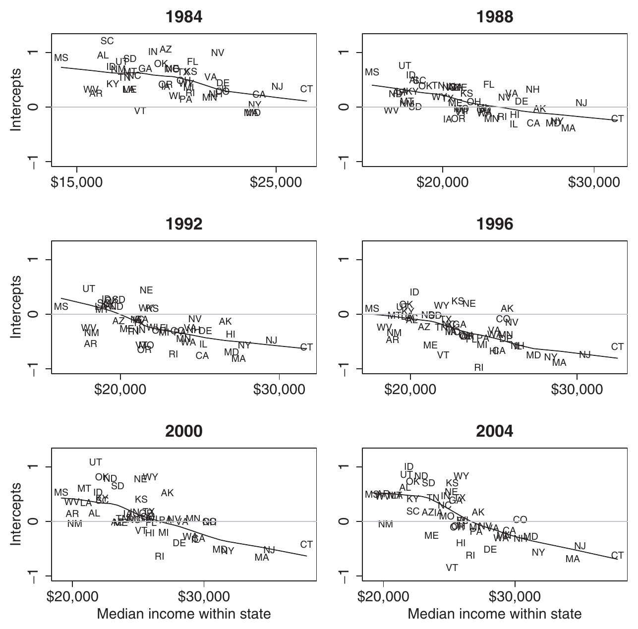
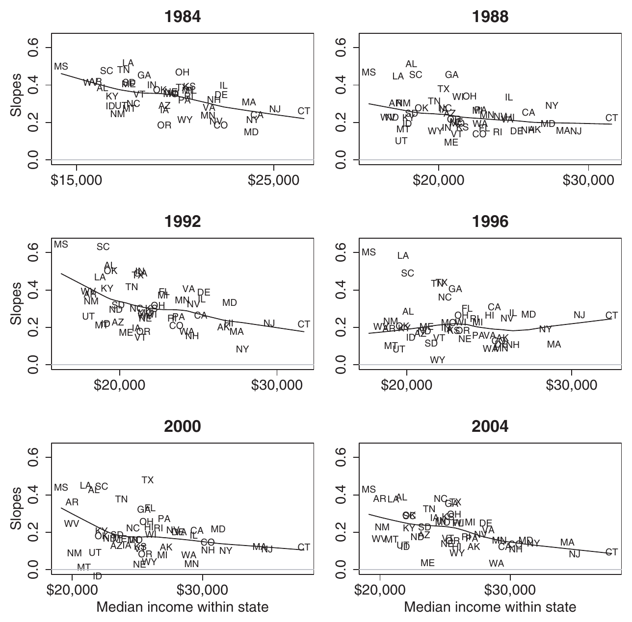
In Part 8, we fit Gelman et al.’s (2007) Model 1 to the CES 2024. They fit the same model to exit polls from each election from 1984 to 2004. (Their Figures 7 and 8, pp. 359–360 [pdf], plot each state’s intercept and slope against state income, one panel per election.) They write that the positive income slopes “have persisted for decades, but only since 1992, and especially since 1996, have systematic differences between rich and poor states become so clear” (p. 357). The paper came out in 2007, so 2004 was its last election.

Now use the ANES for every presidential election from 1952 to 2024. (1948 is the first election in the ANES, but it doesn’t record the respondent’s state.)

# load data; anes voters, 19 elections
anes <- read_csv("https://pos5747.github.io/files/red-state-part9.csv")

• year: the election, 1952 to 2024.
• pc_income: the state’s per-capita personal income in that year, in thousands of 2024 dollars (from the BEA). This is a different measure than Part 8’s state_median_income, which is median household income in 2024 only.
• rs_pc_income: pc_income rescaled (with arm::rescale()) across the 50 states in that year.
• income: the five-point income scale, −2 to 2.
• vote_rep: 1 if the respondent reported voting for the Republican candidate after the election and 0 if they reported voting for the Democrat.

The ANES is small. Each election has 729 to 5,947 voters in 28 to 50 states, and many states have only a handful of voters in a given election. Rather than fit Part 8’s model to each election separately, fit one model that pools across elections.

\[ \begin{aligned} \Pr(\text{vote\_rep}_i = 1) &= \operatorname{logit}^{-1}(\alpha_{s[i]t[i]} + \beta_{s[i]t[i]} \, \text{income}_i) \\ \alpha_{st} &= \gamma_{0t} + \gamma_{1t} z_{st} + \eta^{\alpha}_s + \eta^{\alpha}_{st} \\ \beta_{st} &= \delta_{0t} + \delta_{1t} z_{st} + \eta^{\beta}_s + \eta^{\beta}_{st} \end{aligned} \]

• \(s[i]\) is the state of voter \(i\), \(t[i]\) is the election, and \(z_{st}\) is rs_pc_income.
• Each election has its own four coefficients, \(\gamma_{0t}\), \(\gamma_{1t}\), \(\delta_{0t}\), and \(\delta_{1t}\). Across elections, these four are multivariate normal, so each election’s estimates are pulled toward the average across elections. This is the part of the model that pools across time.
• \((\eta^{\alpha}_s, \eta^{\beta}_s)\) is state \(s\)’s deviation from the lines in every election. (It has no \(t\) subscript, so it’s the same in every election.) \((\eta^{\alpha}_{st}, \eta^{\beta}_{st})\) is its deviation in election \(t\) only. Both pairs are bivariate normal with mean zero.
• In brm(), the formula is vote_rep ~ rs_pc_income * income + (1 + rs_pc_income * income | year) + (1 + income | state_name) + (1 + income | state_name:year).

The model makes two simplifications worth considering. First, it treats the elections as exchangeable. It doesn’t know that 1952 is closer to 1956 than to 2024. (Though we could build that into the model!) Second, the state deviations \((\eta^{\alpha}_s, \eta^{\beta}_s)\) are the same from 1952 to 2024, even though the South moved toward the Republicans over these years. The state-election deviations absorb some of that movement.

1. Fit the model with brm(). Use family = bernoulli, backend = "cmdstanr", chains = 4, cores = 4, iter = 8000, and warmup = 1000. (The fit takes about 20 minutes on a fast desktop.) Check R-hat and the ESS.

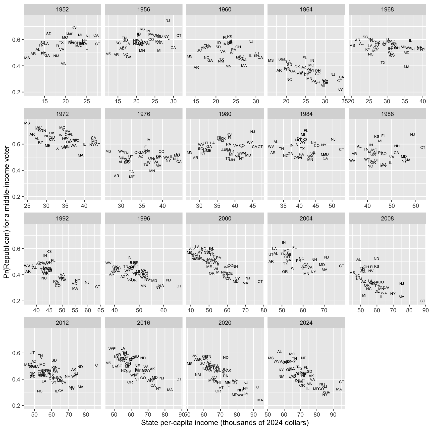
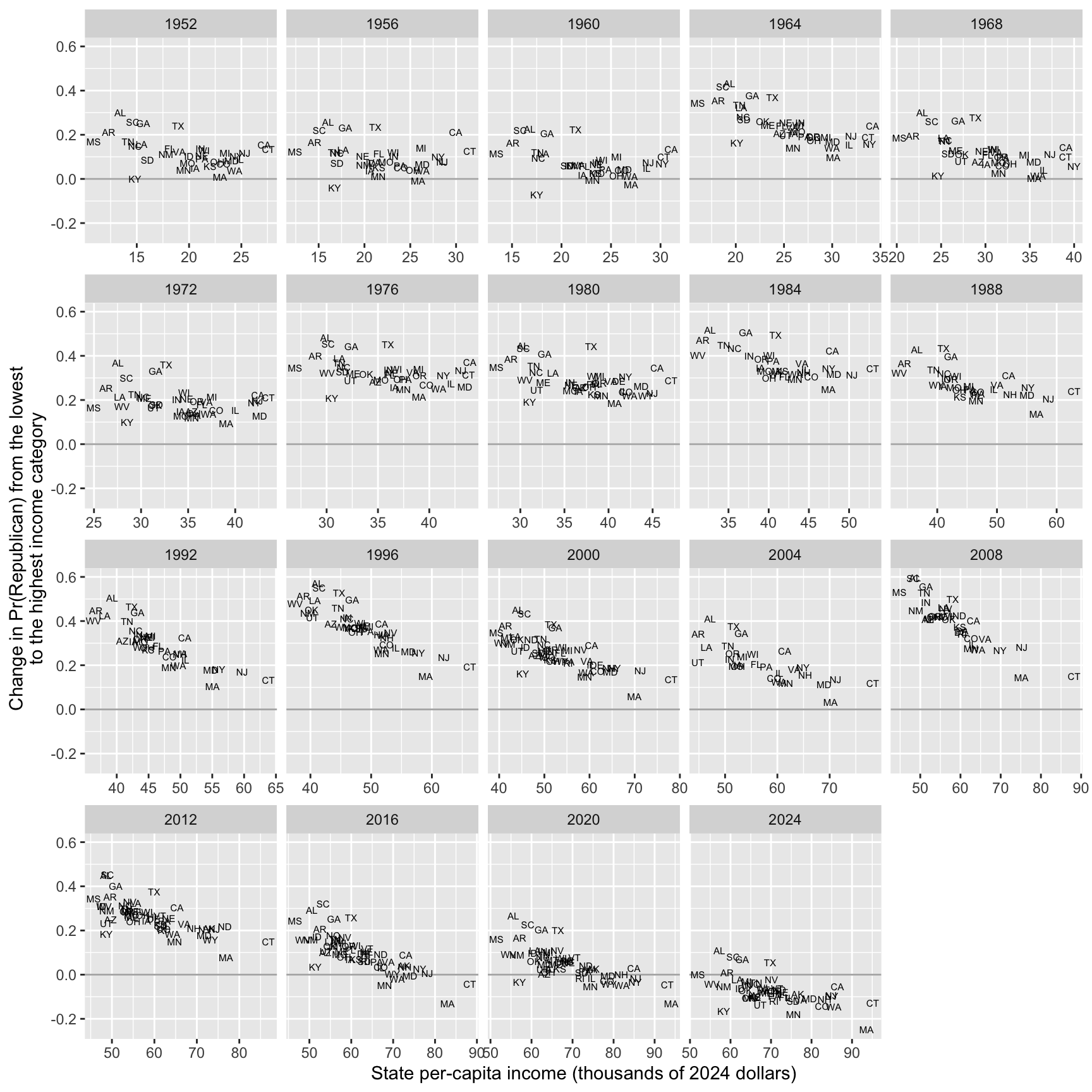
2. For a middle-income voter (income = 0) in each state the ANES sampled in each election, compute (a) the chance of voting for the Republican with predictions() and (b) the change in that chance as income moves from its minimum to its maximum with comparisons(). Then make Part 8’s two plots, with one panel per election: one with the chance on the y-axis and one with the change on the y-axis, both with pc_income on the x-axis and each state’s abbreviation as its point.

3. Interpret the plots and compare them with Gelman et al.’s Figures 7 and 8 (below). Their Figure 7 plots each state’s intercept \(\alpha_s\) against state income, and their Figure 8 plots each state’s income slope \(\beta_s\), for each election from 1984 to 2004. (Their figures are on the log-odds scale and yours are on the probability scale, so compare the patterns, not the numbers.)

   1. In which elections are the rich states more Republican than the poor states? In which are they less Republican? Compare your plot of the chance with their Figure 7.
   2. In which elections does individual income matter more in the poor states than in the rich states? Compare your plot of the change with their Figure 8.
   3. The screenshots below show Figures 7 and 8 from the original paper, which are analogous to the figures you created in (b). How have the patterns changed since 2004?

   

   Figure 7 of Gelman et al. (2007, p. 359): each state’s intercept plotted against state income, with the model fit separately to the exit poll from each election.

   

   Figure 8 of Gelman et al. (2007, p. 360): each state’s income slope plotted against state income, with the model fit separately to the exit poll from each election.

Complete solution

Part 1

fit_rs9 <- brm(vote_rep ~ rs_pc_income * income +
                 (1 + rs_pc_income * income | year) +
                 (1 + income | state_name) +
                 (1 + income | state_name:year),
               data = anes,
               family = bernoulli,
               backend = "cmdstanr",
               iter = 2000,
               warmup = 1000,
               chains = 4,
               cores = 4,
               seed = 1234)

summary(fit_rs9, prob = 0.9)

 Family: bernoulli 
  Links: mu = logit 
Formula: vote_rep ~ rs_pc_income * income + (1 + rs_pc_income * income | year) + (1 + income | state_name) + (1 + income | state_name:year) 
   Data: anes (Number of observations: 30953) 
  Draws: 4 chains, each with iter = 2000; warmup = 1000; thin = 1;
         total post-warmup draws = 4000

Multilevel Hyperparameters:
~state_name (Number of levels: 50) 
                      Estimate Est.Error l-90% CI u-90% CI Rhat Bulk_ESS
sd(Intercept)             0.20      0.04     0.15     0.27 1.01      897
sd(income)                0.09      0.02     0.06     0.13 1.00     1368
cor(Intercept,income)     0.07      0.26    -0.38     0.49 1.00     1018
                      Tail_ESS
sd(Intercept)             1843
sd(income)                1585
cor(Intercept,income)     1767

~state_name:year (Number of levels: 725) 
                      Estimate Est.Error l-90% CI u-90% CI Rhat Bulk_ESS
sd(Intercept)             0.28      0.02     0.24     0.31 1.00     1135
sd(income)                0.05      0.03     0.01     0.09 1.01      360
cor(Intercept,income)    -0.35      0.38    -0.91     0.35 1.00     1609
                      Tail_ESS
sd(Intercept)             2141
sd(income)                 834
cor(Intercept,income)     1681

~year (Number of levels: 19) 
                                      Estimate Est.Error l-90% CI u-90% CI Rhat
sd(Intercept)                             0.37      0.07     0.27     0.50 1.00
sd(rs_pc_income)                          0.32      0.08     0.21     0.46 1.00
sd(income)                                0.18      0.04     0.12     0.24 1.00
sd(rs_pc_income:income)                   0.08      0.05     0.01     0.16 1.01
cor(Intercept,rs_pc_income)               0.48      0.21     0.08     0.79 1.00
cor(Intercept,income)                    -0.15      0.23    -0.51     0.22 1.00
cor(rs_pc_income,income)                  0.09      0.25    -0.34     0.48 1.01
cor(Intercept,rs_pc_income:income)        0.33      0.34    -0.32     0.81 1.00
cor(rs_pc_income,rs_pc_income:income)     0.39      0.35    -0.30     0.86 1.00
cor(income,rs_pc_income:income)          -0.28      0.35    -0.77     0.37 1.00
                                      Bulk_ESS Tail_ESS
sd(Intercept)                              619     1572
sd(rs_pc_income)                          1088     1708
sd(income)                                1194     1901
sd(rs_pc_income:income)                    758      878
cor(Intercept,rs_pc_income)               1384     1955
cor(Intercept,income)                     1071     1791
cor(rs_pc_income,income)                   727     1281
cor(Intercept,rs_pc_income:income)        2596     2070
cor(rs_pc_income,rs_pc_income:income)     1909     1980
cor(income,rs_pc_income:income)           2508     2712

Regression Coefficients:
                    Estimate Est.Error l-90% CI u-90% CI Rhat Bulk_ESS Tail_ESS
Intercept              -0.01      0.10    -0.18     0.15 1.01      374      529
rs_pc_income           -0.09      0.10    -0.26     0.08 1.01      752     1391
income                  0.23      0.05     0.15     0.30 1.00     1001     1465
rs_pc_income:income    -0.08      0.05    -0.15     0.00 1.01     1371     2061

Draws were sampled using sample(hmc). For each parameter, Bulk_ESS
and Tail_ESS are effective sample size measures, and Rhat is the potential
scale reduction factor on split chains (at convergence, Rhat = 1).

R-hat is 1.00 for every parameter (the largest is 1.002), and the smallest bulk ESS is about 2,640 (the intercept). No divergent transitions.

Part 2

# a middle-income voter in each state the anes sampled in each election
typical <- anes |>
  distinct(year, state_name, state_abbr, pc_income, rs_pc_income) |>
  mutate(income = 0)

# the chance of voting for the Republican
pr <- predictions(fit_rs9, newdata = typical, conf_level = 0.9)

# the change in the chance as income moves from its minimum (-2) to its maximum (2)
cmp <- comparisons(fit_rs9, variables = list(income = "minmax"), newdata = typical, conf_level = 0.9)

# combine into one data frame, one row per state-election
qi <- typical |>
  mutate(pr_rep = pr$estimate,
         change = cmp$estimate)

# the chance of voting for the Republican by state income
ggplot(qi, aes(x = pc_income, y = pr_rep, label = state_abbr)) +
  geom_text(size = 2) +
  facet_wrap(vars(year), scales = "free_x") +
  labs(x = "State per-capita income (thousands of 2024 dollars)",
       y = "Pr(Republican) for a middle-income voter")

# the change in the chance by state income
ggplot(qi, aes(x = pc_income, y = change, label = state_abbr)) +
  geom_hline(yintercept = 0, color = "grey70") +
  geom_text(size = 2) +
  facet_wrap(vars(year), scales = "free_x") +
  labs(x = "State per-capita income (thousands of 2024 dollars)",
       y = "Change in Pr(Republican) from the lowest\nto the highest income category")

Part 3

Gelman et al.’s Figures 7 and 8 show three patterns from 1984 to 2004:

1. Poor states are more Republican than rich states.
2. Richer voters are more Republican in every state.
3. Income matters more in poor states.

After 2004:

1. Poor states are still more Republican than rich states. In every election from 2008 to 2024, the chance that a middle-income voter votes Republican falls as state income rises.
2. By 2024, the change from the lowest to the highest income category is negative in 43 of the 49 states. Richer voters are no longer more Republican within most states.
3. Income still has a more positive (less negative?) effect in poor states. But the change now runs from about zero in the poor states to negative in the rich states, rather than being positive everywhere.