A Perspective on Practices

12+ years post-PhD

An Agenda

Claim 1: As political methodologists, we should place greater focus on critiques and refinements of current common practices rather than on pushing the bleeding edge forward. Both are great, but the former is undervalued. Examples: textbooks, software, tutorial-style papers, and reviews of current practices.

• Andrew Gelman’s textbooks (and blog) versus his articles.
• Stan + {brms} + {marginaleffects}
• Ornstein (2023): “It covers the history of MRP, recent advances, an example analysis with code, and concludes with a discussion of best practices and limitations of the approach.”
• Lal et al. (2024): “we replicate 67 articles published in three top political science journals from 2010 to 2022 and identify several concerning patterns… We provide a checklist and software to help researchers avoid these pitfalls and improve their practice.”

Claim 2: As a discipline, we should value description more!

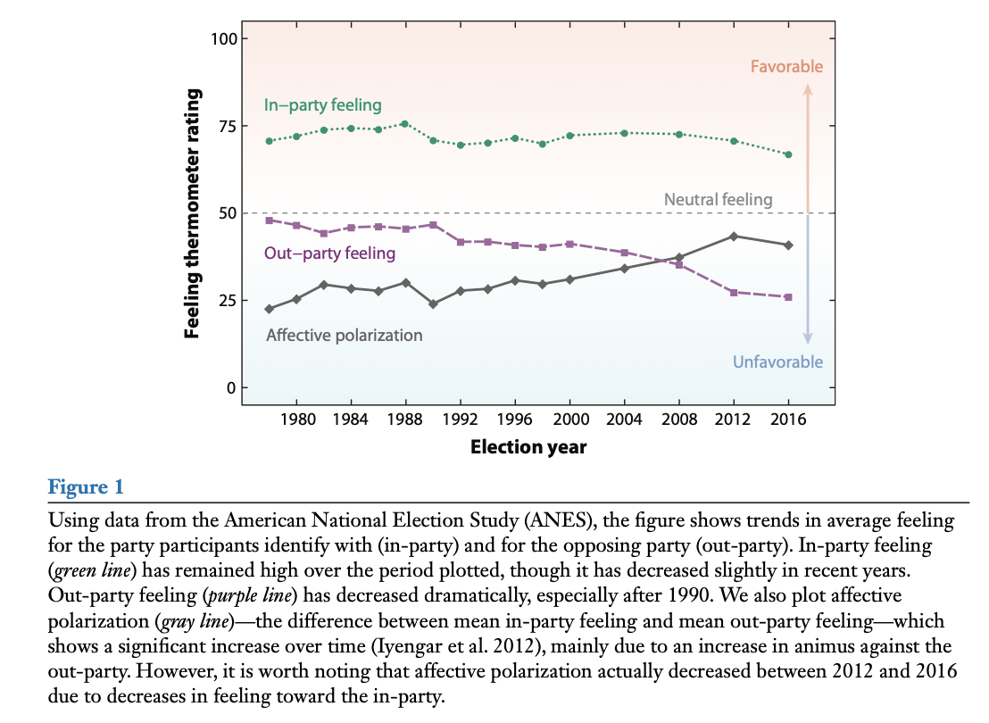
• Iyengar et al. (2019): “Ordinary Americans increasingly dislike and distrust those from the other party.”
• Holliday et al. (2024): “Democrats and Republicans overwhelmingly and consistently oppose norm violations and partisan violence—even when their own representatives engage in antidemocratic actions.”
• FOWLER et al. (2022): “We find there are many genuine moderates in the American electorate. Nearly three in four survey respondents’ issue positions are well described by a single left–right dimension, and most of those individuals have centrist views.”
• Little and Meng (2024): “Despite the general narrative that the world is in a period of democratic decline [around the world], there have been surprisingly few empirical studies that assess whether this is systematically true.”

My description of political science: An investigation of how we can intervene in the world to make the world a better place. (Not everyone agrees!)

• Explicit normative goals or criteria. (We don’t have to agree on these or how to trade these off against each other.)
• Understand the causal effects of potential interventions.
• A clear description of the world we are intervening into.

Advice

Avoid the race to a regression.

Claim 3: As a discipline, we should be more mindful of noise.

• Important consequences for you. You want to conduct studies that allow you to make meaningful claims at the end. (After all, they take hundreds of hours!)
• Important consequences for literatures.

The Importance of Claims and Tests

At the core of empirical research, we have claims about the world. These can be descriptive or causal.

Example: “Ordinary Americans increasingly dislike and distrust those from the other party” (Iyengar et al. 2019).

Generally, we want to make empirical claims when we think they are correct (i.e., when we can rule out other claims).

Hypothesis Testing

Research Hypothesis

A researcher posits a theoretically interesting hypothesis \(H_r\), sometimes called the “alternative” or “research” hypothesis.

Definition 1 A research hypothesis \(H_r\) is a claim that the parameter of interest \(\theta\) lies in a specific region \(B \subset \mathbb{R}\).

Typical forms in political science:

• \(H_r: \theta > 0\) (positive effect)
• \(H_r: \theta < 0\) (negative effect)
• \(H_r: \theta > m\), where \(m\) is a substantively meaningful threshold
• \(H_r: \theta \in (-m,m)\) to test for negligible effects (see Rainey 2014).

Null Hypothesis

Each research hypothesis implies a null hypothesis.

Definition 2 \(H_0\) claims that \(\theta \in B^C\) (i.e., the research hypothesis is false).

Note: The null does not always state “no effect.”
For example, if \(H_r: \theta > 1\), then \(H_0: \theta \le 1\).

Testing Hypotheses

A test statistic summarizes evidence against the null hypothesis.

Definition 3 A test statistic \(T(\mathbf{x}) \in [0,\infty)\) increases (or decreases) with evidence against \(H_0\).

A hypothesis test divides possible values of \(T\) into:

• Rejection region \(R\) → reject \(H_0\)
• Non-rejection region \(R^C\) → fail to reject \(H_0\)

Important: Failure to reject \(H_0\) means ambiguous evidence, not evidence that \(H_0\) is true.

Errors in Hypothesis Testing

Two types of errors:

Name	Label	Longer Label	Error Rate	Person in Charge
Type I	“False Positive”	You claim that your research hypothesis is true, but it is not true.	5%	Statistician
Type II	“False Negative” / “Lost Opportunity”	You cannot make a claim about your research hypothesis.	???	You, the researcher

You make an “error” when you make a claim that is false. When we design procedures, we should control the error rate.

\(p\)-Value

Given a test statistic \(T\) (larger values → more evidence against \(H_0\)):

Definition 4 \(p\text{-value} = \max_{\theta \in B^C} P(T(\mathbf{X}) \ge T(\mathbf{x}))\)

“The probability of obtaining data more extreme than the data we actually obtained if the null hypothesis were true.”

Reject \(H_0\) if and only if \(p \le \alpha\) (e.g., \(\alpha = 0.05\)).

\(p\)-values are a beautiful, elegant, and powerful way to make empirical arguments with noisy data. No proposed solution (e.g., Bayes factors, posterior probabilities, \(S\)-values) solves the “problems” with \(p\)-values.

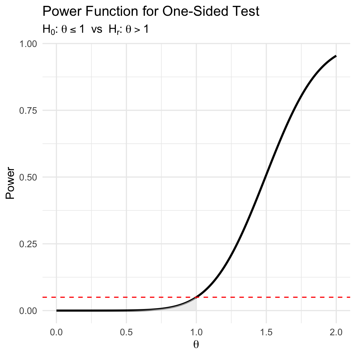
Power and Size

Definition 5 The power function gives \(\Pr(\text{reject } H_0 \mid \theta)\).

We want:

• Low rejection probability when \(\theta \in B^C\)
• High rejection probability when \(\theta \in B\)

Definition 6 A size-\(\alpha\) test has maximum Type I error probability equal to \(\alpha\).

Example: Testing a Substantively Meaningful Effect

Let \(\theta = \mu_1 - \mu_2\).

• Research hypothesis: \(H_r : \theta > 1\)
  
• Null hypothesis: \(H_0 : \theta \le 1\)

Test statistic: \(T = \frac{\hat{\theta} - 1}{\text{SE}(\hat{\theta})}\)

\(p\)-value: \(p = P(Z \ge T)\) where \(Z \sim N(0,1)\).

Reject \(H_0\) if \(p \le 0.05\). Otherwise, evidence is ambiguous.

Confidence Intervals and Hypothesis Tests

One way to create a confidence interval is to invert a hypothesis test.

For example, suppose a hypothesis \(H_r: \theta > m\).

• For any particular \(m\), we can compute a \(p\)-value and will either reject the null hypothesis or not.
• We can collect the \(m\) for which we rejected the null hypothesis into a collection; and collect the \(m\) for which we did not reject the null hypothesis into a separate collection.
• For the usual z-test (or t-test), there will be a single value \(m^*\) that partitions the parameter space \(\Theta\) into those (smaller) \(m \leq m^*\) that can be rejected and those (larger) \(m > m^*\) that cannot be rejected.
• If we set \(m^* = L\), then \([L, \infty)\) is a 95% one-sided confidence interval.
• \(L\) tells us the smallest \(\theta\) that we cannot reject with a one-sided, size-0.05 test.

We could similarly do this for \(H_r: \theta < m\).

• Find 95% one-sided confidence interval \((-\infty, U]\).
• \(U\) tells us the largest \(\theta\) that we cannot reject with a one-sided, size-0.05 test.

If we use the \(L\) and the \(U\) from above, we have a 90% CI.

The endpoints of this 90% CI tell us…

• the smallest \(\theta\) that we cannot reject with a one-sided, size-0.05 test.
• the largest \(\theta\) that we cannot reject with a one-sided, size-0.05 test.

Warning

Be careful of your claim!

• “\(X\) has a large, substantively meaningful effect on \(E(Y)\).”
  • Can you reject all substantively negligible effects?
  • Is \(L\) in the 90% CI substantively meaningful?
• “\(X\) has no effect on \(E(Y)\).”
  • Can you reject all non-zero effects? (No! Never.)
  • Is \(L\) in the 90% CI substantively meaningful?
  • Is \(U\) in the 90% CI substantively meaningful?
    

Advice

Only make a claim if the claim holds for the entire confidence interval.

Read Rainey (2014) and McCaskey and Rainey (2015).

Exam Question

I like to say: “Only make a claim if the claim holds for the entire confidence interval.” Using the arguments from Rainey (2014) and McCaskey and Rainey (2015), give two examples of how current practice deviates from this advice. Explain why these deviations matter. Explain a how my advice applies to these two sitations.

Examples:

1. McCaskey and Rainey (2015): Claiming “substantively significant” if the point estimate is meaningful (and statistically significant).
2. Rainey (2014): Claiming “no effect” when an estimate is not statistically significant.

I like 90% CIs for principled reasons—it corresponds to a size-0.05 test for the claims we typically make. But others prefer 95% CIs. That’s fine, too.

Testing for Negligible Effects

I write about this in Rainey (2014).

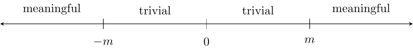
Define a threshold \(m > 0\) for the smallest substantively meaningful effect.

Definition 7 \(H_r : \theta \in (-m, m)\) = effect is negligible.

Definition 8 \(H_0 : \theta \le -m \text{ or } \theta \ge m\) = effect is meaningfully large (+ or -).

Use the two one-sided tests (TOST) procedure.

• Test both \(H_{r1}: \theta < m\) and \(H_{r2}: \theta > -m\).
• We need to reject both null hypotheses.

We reject \(H_0\) if the \((1-2\alpha)\) confidence interval lies entirely inside \((-m,m)\). A 90% CI gives you a size-0.05 equivalence test.

Power

• You spend years on a study.
• The chance that you are wasting your time is non-trivial.
• But… this chance can be investigated beforehand.

How to compute power?

• “Power Rules” [preprint]
• G*Power [web]
• {DeclareDesign} [book]
• MC simulations

The MDE: What effect can I detect with 80% or 95% power?

You want your standard error to be about \(\frac{m}{3.3}\).

• This gives you 95% power to detect an effect of \(m\).
• This (nearly) guarantees that the 90% CI will include at most two regions.

For your research area, you should have this diagram in mind, an \(m\) in mind, and the implied target SE in mind.

In talks, you might have heard me ask about the scale of the estimates. I usually ask how an estimate should be interpreted. But I’m looking at the SE when I ask that question, because I’m constructing this picture in my mind—I want to know how the SE compares to \(m\).

The Consequences of Power

# parameters
sd_y <- 1.0
ate <- 0.1
N <- c(100, 500, 2500, 4500)

# compute power
se <- 2*sd_y/(sqrt(N))  # rule 3 from "power rules"
pwr <- 1-pnorm(1.64 - ate/se); pwr  # rule 2

[1] 0.1271432 0.3008470 0.8051055 0.9567450

MC Simulation

# do MC simulation
set.seed(123)
res_list <- NULL
iter <- 1
for (i in 1:10000) {
  for (j in 1:length(N)) {
    # simulate data and fit model
    y0 <- rnorm(N[j]/2, mean = 0, sd = sd_y)
    y1 <- rnorm(N[j]/2, mean = 0 + ate, sd = sd_y)
    fit <- t.test(y1, y0, conf.level = 0.90)
    # store results
    res_list[[iter]] <- list(
      study_id = i,
      N = N[j],
      pwr = pwr[j],
      est = fit$estimate[1] -fit$estimate[2] ,
      l = fit$conf.int[1],
      u = fit$conf.int[2]
    )
    iter <- iter + 1
  }
}
res <- bind_rows(res_list) 

res |>
  group_by(N, pwr) |>
  summarize(n_mc = n(), mc_pwr = mean(l > 0))

# A tibble: 4 × 4
# Groups:   N [4]
      N   pwr  n_mc mc_pwr
  <dbl> <dbl> <int>  <dbl>
1   100 0.127 10000  0.123
2   500 0.301 10000  0.298
3  2500 0.805 10000  0.804
4  4500 0.957 10000  0.955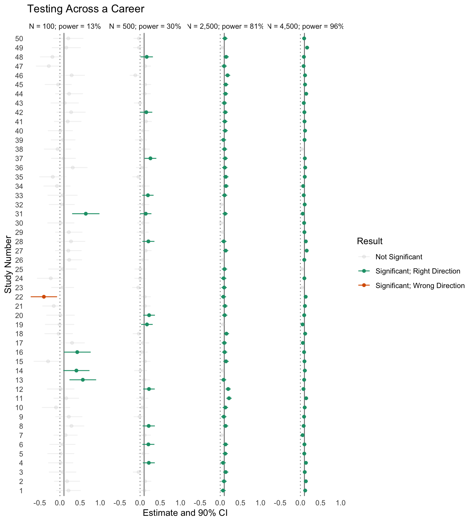

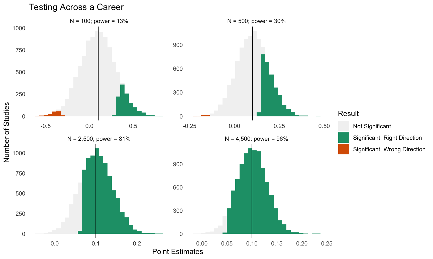
When you test with low power, you make three mistakes:

1. When you do “get it right” you are guaranteed to have “wildly wrong” estimates.
2. You often get it “wildly wrong” in the wrong direction.
3. You often waste your time.

See Gelman and Carlin (2014).

Literatures

What are the implications for literatures if we have 100s of researchers conducting poorly-powered studies and authors, editors, and reviewers filtering on statistical significance?

So what is observed power in political science?

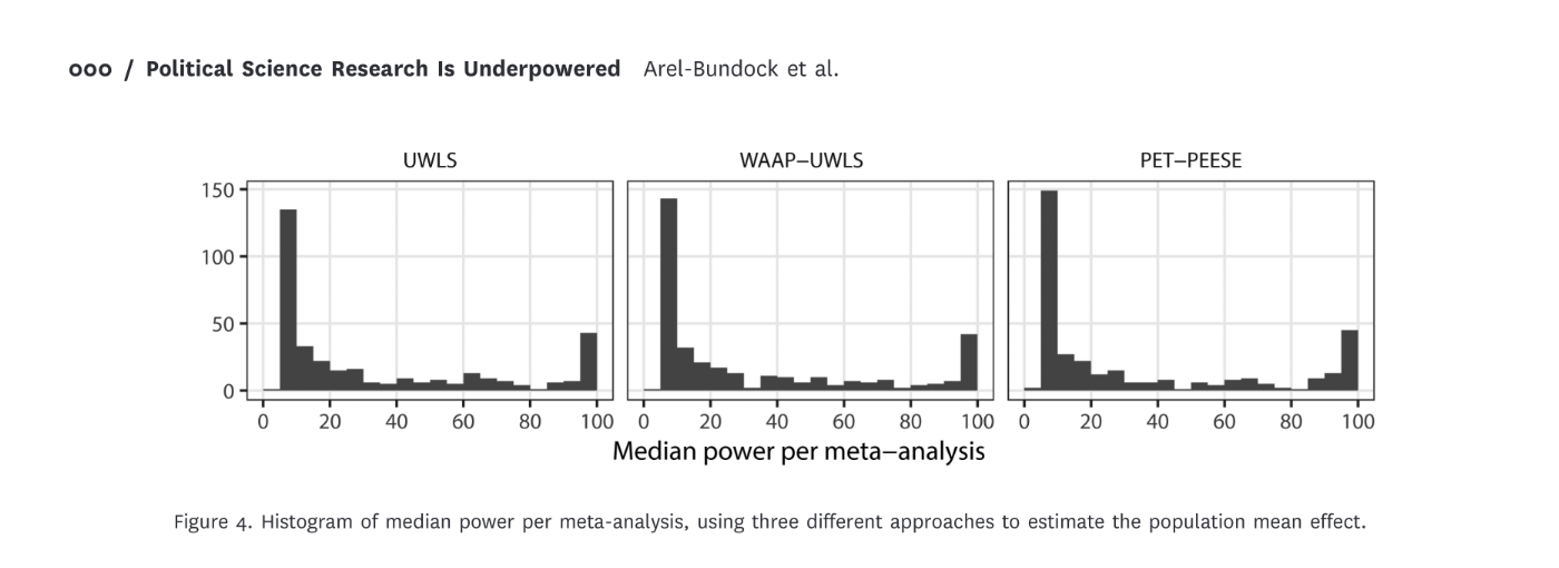
Arel-Bundock et al.

“Under generous assumptions, we show that quantitative research in political science is greatly underpowered: the median analysis has about 10% power, and only about 1 in 10 tests have at least 80% power to detect the consensus effects reported in the literature.”

Is this okay? Tragic? Desirable?

Exam Question

You are an editor of a journal and have received two thoughtful reviews for a well-done survey experiment. While previous work suggests that a treatment should have a positive effect, this new paper on your desk suggests that the treatment has a negative effect and they find a statistically significant negative effect.

• Reviewer A notes that the sample size is small. They cite Gelman and Carlin (2014) and Arel-Bundock et al. (2025) and suggest that the journal shouldn’t publish underpowered work.
• Reviewer B notes that while the sample size is small, the authors’ test protects them against Type I errors as usual (in the sense that \(\Pr(\text{make claim} \mid \text{claim is false}) \leq 0.05\)). (Recall that power relates to Type II errors, which the authors definitely haven’t made here.)

1. Explain each perspective more fully.
2. How do you adjudicate between these perspectives? Describe the tradeoffs between a policy of (1) requiring that all papers be well-powered and (2) not considering the power once data have been collected. Which of these policies would you advocate for?
3. Years later, you are no longer an editor, but have accumulated some formal and informal power in the discipline. You decide to return to this issue. What norms, practices, or rules might you change to address this issue?

References

Arel-Bundock, Vincent, Ryan C. Briggs, Hristos Doucouliagos, Marco M. Aviña, and T. D. Stanley. 2025. “Quantitative Political Science Research Is Greatly Underpowered.” The Journal of Politics, September, 000–000. https://doi.org/10.1086/734279.

FOWLER, ANTHONY, SETH J. HILL, JEFFREY B. LEWIS, CHRIS TAUSANOVITCH, LYNN VAVRECK, and CHRISTOPHER WARSHAW. 2022. “Moderates.” American Political Science Review 117 (2): 643–60. https://doi.org/10.1017/s0003055422000818.

Gelman, Andrew, and John Carlin. 2014. “Beyond Power Calculations.” Perspectives on Psychological Science 9 (6): 641–51. https://doi.org/10.1177/1745691614551642.

Holliday, Derek E., Shanto Iyengar, Yphtach Lelkes, and Sean J. Westwood. 2024. “Uncommon and Nonpartisan: Antidemocratic Attitudes in the American Public.” Proceedings of the National Academy of Sciences 121 (13). https://doi.org/10.1073/pnas.2313013121.

Iyengar, Shanto, Yphtach Lelkes, Matthew Levendusky, Neil Malhotra, and Sean J. Westwood. 2019. “The Origins and Consequences of Affective Polarization in the United States.” Annual Review of Political Science 22 (1): 129–46. https://doi.org/10.1146/annurev-polisci-051117-073034.

Lal, Apoorva, Mackenzie Lockhart, Yiqing Xu, and Ziwen Zu. 2024. “How Much Should We Trust Instrumental Variable Estimates in Political Science? Practical Advice Based on 67 Replicated Studies.” Political Analysis 32 (4): 521–40. https://doi.org/10.1017/pan.2024.2.

Little, Andrew T., and Anne Meng. 2024. “Measuring Democratic Backsliding.” PS: Political Science & Politics 57 (2): 149–61. https://doi.org/10.1017/s104909652300063x.

McCaskey, Kelly, and Carlisle Rainey. 2015. “Substantive Importance and the Veil of Statistical Significance.” Statistics, Politics and Policy 6 (1-2). https://doi.org/10.1515/spp-2015-0001.

Ornstein, Joseph T. 2023. “Getting the Most Out of Surveys: Multilevel Regression and Poststratification.” In, 99–122. Springer International Publishing. https://doi.org/10.1007/978-3-031-12982-7_5.

Rainey, Carlisle. 2014. “Arguing for a Negligible Effect.” American Journal of Political Science 58 (4): 1083–91. https://doi.org/10.1111/ajps.12102.