Interaction

Interaction means: the effect* of \(X\) on \(Y\) depends on the value of some moderating variable \(Z\).

The problem:

we can have interaction on the scale of the linear predictor \(\eta = \beta_0 + \beta_1 x_1 + ... + \beta_k x_k\).
we can have interaction on the scale of the outcome \(E(Y) = g^{-1}(\eta)\).

It isn’t clear which we should care about.
One does not imply the other.
They can even go in opposite directions.

Why the Distinction Matters

Latent Scale \(\eta_i\)

\(\eta_i\) is unbounded and linear in the parameters.
Only the product term can create interaction on this scale.
For the model \(\eta_i = \beta_0 + \beta_1 X_i + \beta_2 Z_i + \beta_3 (X_i Z_i) + \dots\), interaction only exists when \(\frac{\partial^2 \eta_i}{\partial X \partial Z} = \beta_3 \neq 0\).

Probability Scale \(\Pr(Y_i=1)\)

The inverse link \(g^{-1}(\cdot)\) is nonlinear and S-shaped.
Even if \(\beta_3 = 0\) (or no product term is included), the effect of \(X\) on \(\Pr(Y)\) varies with \(Z\) because \(\frac{\partial \Pr(Y_i)}{\partial X} = \frac{d g^{-1}(\eta_i)}{d\eta_i} \cdot \frac{\partial \eta_i}{\partial X}\).
Since \(\frac{d g^{-1}(\eta)}{d\eta}\) depends on \(\eta\), any variable that shifts \(\eta\) affects instantaneous marginal effects.
This follows from compression, where effects shrink as \(\Pr(Y)\) approaches \(0\) or \(1\).
Thus, interaction on the probability scale may occur with or without a product term. It can even have the opposite effect as the product term.

Interaction on the Latent Scale

This scale corresponds to hypotheses explicitly about the latent index (e.g., linear effects on an underlying utility or propensity).

This works just like linear regression, where \(\eta_i = \beta_0 + \beta_1 X_i + \beta_2 Z_i + \beta_3 (X_i Z_i) + \dots\)

Definition

Interaction on the latent scale exists when \(\frac{\partial^2 \eta_i}{\partial X \partial Z} = \beta_3 \neq 0\).

Instantaneous Marginal Effect of \(X\) on \(\eta_i\)

\[ \frac{\partial \eta_i}{\partial X} = \beta_1 + \beta_3 Z_i. \]

First Difference

For a discrete change in \(X\),

\[ \Delta \eta_i = \beta_3(Z_{hi} - Z_{lo}). \]

Interaction on the Probability Scale

We can measure interaction on the probability scale with

second derivatives (cross-partials)
second differences

Approach I: Using Derivatives

Definition of Interaction I (Derivatives)

Interaction on the probability scale is present when

\[ \frac{\partial^2 \Pr(Y_i)}{\partial X \partial Z} \neq 0. \]

Depends on the mixture of:

Latent interaction (\(\beta_3 \neq 0\))
Nonlinearity of the inverse link (\(g^{-1}\)).

I don’t find these instantaneous marginal effects useful, except when they are constant.

Approach II: Using Differences

For a discrete change in \(X\) at a fixed value of \(Z\), define the first difference as

\[ \Delta_X(Z) = \Pr(Y=1 \mid X_{hi}, Z) - \Pr(Y=1 \mid X_{lo}, Z). \]

And define the second difference as

\[ \Delta\Delta = \big[ \Pr(Y \mid X_{hi}, Z_{hi}) - \Pr(Y \mid X_{lo}, Z_{hi}) \big] - \big[ \Pr(Y \mid X_{hi}, Z_{lo}) - \Pr(Y \mid X_{lo}, Z_{lo}) \big]. \]

Definition of Interaction II (Differences)**

If \(\Delta\Delta \neq 0\), the effect of \(X\) changes when \(Z\) changes.

Theoretical Rationale

When to Theorize on the Latent Scale

The theory concerns an unobserved continuous index (e.g., utility, evaluation, propensity).

When to Theorize on the Probability Scale

The theory concerns changes in probability, not the latent index.

Important: the model’s compression must be part of the theory—you must theorize interaction because of ceiling and floor effects.

My Take

We are left with no good default.

Theories are rarely precise enough to distinguish between these in any obvious way.
To the extent they do, they either:
- Build in floor or ceiling effects in not-super-interesting ways (e.g., contiguity and democracy).
- Have an explicit latent utility interpretation (e.g., spatial voting).

Two Claims

These pull us in opposite directions.

Most theories (in my view) vaguely refer to unbounded notions of the outcome.
Most readers expect estimates on the scale of the outcome (probability scale, in this case).

Suggestion

When you are computing quantities of interest, work on the scale of the outcome unless you have a great reason to do otherwise (e.g., spatial models).
When you are theorizing, remain mindful of compression. Go out of your way to explicitly think about what happens as events become very likely or unlikely.

Example

In order to turn out to vote, you need to feel like you have a stake in society.

There are two ways to obtain this feeling:

A financial stake.
A civic stake, mainly developed from education.

If you lack a stake in society, then you tend not to vote. If you have a stake in society, then you tend to vote. Importantly, these two stakes are substitutes—you just need one.

Load our data.

turnout <- ZeligData::turnout |>
  glimpse()

Rows: 2,000
Columns: 5
$ race    <fct> white, white, white, white, white, white, white, white, white,…
$ age     <int> 60, 51, 24, 38, 25, 67, 40, 56, 32, 75, 46, 52, 22, 60, 24, 30…
$ educate <dbl> 14, 10, 12, 8, 12, 12, 12, 10, 12, 16, 15, 12, 12, 12, 14, 10,…
$ income  <dbl> 3.3458, 1.8561, 0.6304, 3.4183, 2.7852, 2.3866, 4.2857, 9.3205…
$ vote    <int> 1, 0, 0, 1, 1, 1, 0, 1, 1, 1, 1, 1, 0, 0, 1, 1, 1, 1, 1, 1, 1,…

And fit two models.

# no product term; scale sets mean = 0 and SD = 1
f <- vote ~ educate + income
fit <- glm(f, data = turnout, family = binomial)

# product term
f2 <- vote ~ educate*income
fit2 <- glm(f2, data = turnout, family = binomial)

library(marginaleffects)

grid <- crossing(educate = unique(turnout$educate), 
                 income = unique(turnout$income)) |>
  glimpse()

Rows: 3,720
Columns: 2
$ educate <dbl> 0, 0, 0, 0, 0, 0, 0, 0, 0, 0, 0, 0, 0, 0, 0, 0, 0, 0, 0, 0, 0,…
$ income  <dbl> 0.0000, 0.1544, 0.1727, 0.1936, 0.2071, 0.2162, 0.2253, 0.2364…

p <- predictions(fit2, newdata = grid) |>
  glimpse()

Rows: 3,720
Columns: 9
$ rowid     <int> 1, 2, 3, 4, 5, 6, 7, 8, 9, 10, 11, 12, 13, 14, 15, 16, 17, 1…
$ estimate  <dbl> 0.3278163, 0.3313963, 0.3318219, 0.3323084, 0.3326228, 0.332…
$ p.value   <dbl> 0.013616537, 0.012327574, 0.012183909, 0.012022241, 0.011919…
$ s.value   <dbl> 6.198496, 6.341967, 6.358879, 6.378150, 6.390571, 6.398930, …
$ conf.low  <dbl> 0.2161033, 0.2224302, 0.2231801, 0.2240365, 0.2245896, 0.224…
$ conf.high <dbl> 0.4631578, 0.4620251, 0.4619032, 0.4617673, 0.4616815, 0.461…
$ educate   <dbl> 0, 0, 0, 0, 0, 0, 0, 0, 0, 0, 0, 0, 0, 0, 0, 0, 0, 0, 0, 0, …
$ income    <dbl> 0.0000, 0.1544, 0.1727, 0.1936, 0.2071, 0.2162, 0.2253, 0.23…
$ df        <dbl> Inf, Inf, Inf, Inf, Inf, Inf, Inf, Inf, Inf, Inf, Inf, Inf, …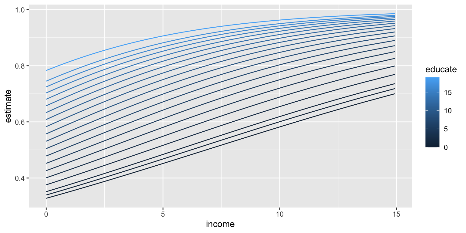

ggplot(p, aes(x = income, y = estimate, color = educate, group = educate)) + 
  geom_line()

# effect of educate moving from 25th to 75th percentile
c <- comparisons(fit2, 
                 variables = list(educate = "iqr"),
                 newdata = datagrid(income = unique)) |>
  glimpse()

Rows: 186
Columns: 16
$ rowid        <int> 1, 2, 3, 4, 5, 6, 7, 8, 9, 10, 11, 12, 13, 14, 15, 16, 17…
$ term         <chr> "educate", "educate", "educate", "educate", "educate", "e…
$ contrast     <chr> "Q3 - Q1", "Q3 - Q1", "Q3 - Q1", "Q3 - Q1", "Q3 - Q1", "Q…
$ estimate     <dbl> 0.09759300, 0.09761655, 0.09761716, 0.09761728, 0.0976170…
$ std.error    <dbl> 0.02299989, 0.02205167, 0.02194130, 0.02181579, 0.0217350…
$ statistic    <dbl> 4.243193, 4.426720, 4.449014, 4.474616, 4.491233, 4.50246…
$ p.value      <dbl> 2.203614e-05, 9.567696e-06, 8.626521e-06, 7.654887e-06, 7…
$ s.value      <dbl> 15.46977, 16.67340, 16.82279, 16.99519, 17.10757, 17.1837…
$ conf.low     <dbl> 0.05251403, 0.05439608, 0.05461300, 0.05485911, 0.0550171…
$ conf.high    <dbl> 0.1426720, 0.1408370, 0.1406213, 0.1403754, 0.1402169, 0.…
$ educate      <dbl> 12.06675, 12.06675, 12.06675, 12.06675, 12.06675, 12.0667…
$ vote         <int> 1, 1, 1, 1, 1, 1, 1, 1, 1, 1, 1, 1, 1, 1, 1, 1, 1, 1, 1, …
$ income       <dbl> 0.0000, 0.1544, 0.1727, 0.1936, 0.2071, 0.2162, 0.2253, 0…
$ predicted_lo <dbl> 0.5831084, 0.5888519, 0.5895310, 0.5903063, 0.5908068, 0.…
$ predicted_hi <dbl> 0.6807014, 0.6864684, 0.6871482, 0.6879235, 0.6884238, 0.…
$ predicted    <dbl> NA, NA, NA, NA, NA, NA, NA, NA, NA, NA, NA, NA, NA, NA, N…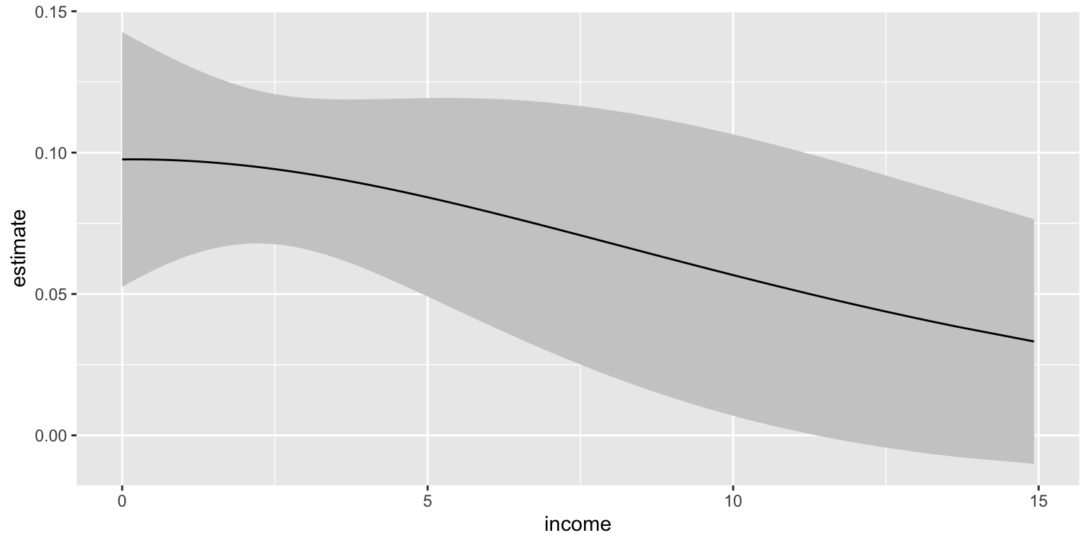

ggplot(c, aes(x = income, y = estimate, ymin = conf.low, ymax = conf.high)) + 
  geom_ribbon(fill = "grey80") + 
  geom_line()

A Formal Test

We need to actually compute the second difference and test whether it’s difference from zero.

Confidence interval.
p-value

p <- predictions(fit2, 
                 variables = list(educate = "iqr", income = "iqr"),
                 newdata = datagrid()) |>
  glimpse()

Rows: 4
Columns: 11
$ rowid     <int> 1, 2, 3, 4
$ rowidcf   <int> 1, 1, 1, 1
$ estimate  <dbl> 0.6463424, 0.7573006, 0.7423496, 0.8403306
$ p.value   <dbl> 1.140540e-21, 8.609417e-27, 2.616875e-31, 1.262546e-91
$ s.value   <dbl> 69.57077, 86.58614, 101.59193, 301.95912
$ conf.low  <dbl> 0.6176103, 0.7170342, 0.7068251, 0.8176278
$ conf.high <dbl> 0.6740549, 0.7934874, 0.7749401, 0.8606888
$ vote      <int> 1, 1, 1, 1
$ educate   <dbl> 10, 10, 14, 14
$ income    <dbl> 1.7443, 5.2331, 1.7443, 5.2331
$ df        <dbl> Inf, Inf, Inf, Inf

p |> 
  select(educate, income, estimate, conf.low, conf.high) |>
  tinytable::tt()

educate	income	estimate	conf.low	conf.high
10	1.7443	0.6463424	0.6176103	0.6740549
10	5.2331	0.7573006	0.7170342	0.7934874
14	1.7443	0.7423496	0.7068251	0.7749401
14	5.2331	0.8403306	0.8176278	0.8606888

# compute the ci and p-value for the 2nd difference
# this is a formal test for interaction on the probability scale
hypotheses(p, hypothesis = "(b4 - b2) - (b3 - b1) = 0")


        Hypothesis Estimate Std. Error      z Pr(>|z|)   S  2.5 % 97.5 %
 (b4-b2)-(b3-b1)=0   -0.013      0.104 -0.125    0.901 0.2 -0.217  0.191

Warning

"b4" isn’t the hi-hi-scenario. It’s just the 4th row in p. If the rows in p change, so to does the meaning of "b4". Be careful!

But…

Here is the test for the model without a product term.

p <- predictions(fit, 
                 variables = list(educate = "iqr", income = "iqr"),
                 newdata = datagrid())

hypotheses(p, hypothesis = "(b4 - b2) - (b3 - b1) = 0")


        Hypothesis Estimate Std. Error         z Pr(>|z|)   S   2.5 %  97.5 %
 (b4-b2)-(b3-b1)=0  -0.0249   1.44e-09 -17233833   <0.001 Inf -0.0249 -0.0249

How can this happen?!?

Also but…

modelsummary::modelsummary(list("No Prod." = fit, "Prod" = fit2))

	No Prod.	Prod
(Intercept)	-0.861	-0.718
	(0.192)	(0.291)
educate	0.118	0.105
	(0.018)	(0.026)
income	0.165	0.105
	(0.026)	(0.096)
educate × income		0.005
		(0.007)
Num.Obs.	2000	2000
AIC	2110.4	2111.9
BIC	2127.2	2134.3
Log.Lik.	-1052.181	-1051.966
F	68.490	44.642
RMSE	0.42	0.42