IRT

Here are the packages we’re using:

# generally useful packages
library(tidyverse)
library(marginaleffects)
library(modelsummary)
library(patchwork)

# for fitting hierarchical models
library(lme4)
library(brms)  # see also rstanarm::stan_lmer()
library(cmdstanr)

# for post-processing simulations
library(tidybayes)

# preferred order (most preferred first):
library(conflicted)
conflict_prefer_all("dplyr", quiet = TRUE)
conflict_prefer_all("tidyr", quiet = TRUE)
conflict_prefer_all("tidybayes", quiet = TRUE)
conflict_prefer_all("brms", quiet = TRUE)
conflict_prefer_all("patchwork", quiet = TRUE)

IRT

This week, I introduce the idea of an IRT model.

This is just one specific type of hierarchical model.

The `answers` data

The answers dataset has answers from hypothetical students to real questions from a recent exam.

question_id_num indexes the 55 questions on the exam.
student_id_num indexes the 100 students who took the exam.
correct_answer indicates (0/1) where the student answered the question correctly.

answers <- read_csv("https://pos5747.github.io/data/example-answers.csv") |>
  glimpse()

Rows: 5,500
Columns: 3
$ student_id_num  <dbl> 1, 1, 1, 1, 1, 1, 1, 1, 1, 1, 1, 1, 1, 1, 1, 1, 1, 1, 1, 1, 1, 1…
$ question_id_num <dbl> 1, 2, 3, 4, 5, 6, 7, 8, 9, 10, 11, 12, 13, 14, 15, 16, 17, 18, 1…
$ correct_answer  <dbl> 1, 1, 1, 1, 1, 1, 1, 1, 1, 1, 1, 1, 1, 1, 0, 1, 1, 1, 1, 1, 1, 1…

Grades on the exam

grades <- answers %>%
  group_by(student_id_num) %>%
  summarize(proportion_correct = mean(correct_answer)) %>%
  mutate(
    letter_grade = cut(
      proportion_correct,
      breaks = c(-Inf, 0.60, 0.63, 0.67, 0.70, 0.73, 0.77, 0.80, 0.83, 0.87, 0.90, 0.93, Inf),
      right = FALSE,  # 0.60 is a D-, not an F
      labels = c("F",  "D-", "D",  "D+", "C-", "C",  "C+", "B-", "B",  "B+", "A-", "A"),
      ordered_result = TRUE
    )
  )

grades |> filter(student_id_num <= 10)

# A tibble: 10 × 3
   student_id_num proportion_correct letter_grade
            <dbl>              <dbl> <ord>       
 1              1              0.909 A-          
 2              2              0.527 F           
 3              3              0.764 C           
 4              4              0.727 C-          
 5              5              0.964 A           
 6              6              0.818 B-          
 7              7              0.818 B-          
 8              8              0.782 C+          
 9              9              0.564 F           
10             10              0.8   B-

Rasch / 1-PL model

Indices

Answers: $n = 1, \dots, N$. ($N = 55 \times 100 = 5{,}500$ in our data.)
Students: $j = 1, \dots, J$. ($J = 100$ in our data.)
Questions: $k = 1, \dots, K$. ($K = 55$ in our data.)

Outcome: $y_{n} \in \{0, 1\}$ indicates whether the $n$th answer is correct.

\[ y_n \sim \text{Bernoulli}(\pi_n) \\ \pi_n = \operatorname{logit}^{-1} \left( \mu + \alpha_{j[n]} - \beta_{k[n]} \right). \]

Parameters

$\pi_n$: the probability that answer $n$ is correct
$\alpha_{j[n]}$: the ability of student $j$ [who is giving the $n$th answer].
- Higher $\alpha_j$ ⇒ more likely to answer correctly; more knowledgeable student.
$\beta_{k[n]}$: the difficulty of question $k$ [which is associated with the $n$th answer].
- Higher $\beta_k$ ⇒ less likely to answer correctly; harder item.
$\mu$: the log-odds of a correct answer for an average student on an average question

Hierarchical Model

\[ \alpha_j \sim N(0,\sigma_\alpha^2)\\ \beta_k \sim N(0,\sigma_\beta^2) \]

Priors

\[ \sigma_\alpha \sim \text{half-Cauchy}(0,1)\\ \sigma_\beta \sim \text{half-Cauchy}(0,1) \]

\[ \mu \sim \text{Cauchy}(0,1). \]

A change from 0 to 1 on the logit scale increases the chance of success from 50% to 73%. A change from 1 to 2 increases the chance of success from 73% to 88%.

plogis(0); plogis(1); plogis(2)

[1] 0.5

[1] 0.731

[1] 0.881

$\sigma_\alpha = 1$ means that the “give or take” on the abilities is about 1.
Suppose an average student has a 73% chance of answering a given question correctly. If $\sigma_\alpha = 1$, then “most” (68%) students have between a 50% and 88% chance of answering correctly. This seems “about right” to me, so I expect $\sigma_\alpha$ to be about 1 (i.e., not 0.1 or 10).
The median of a half-Cauchy is the scale, so I set the scale to the $\sigma_\alpha$ that seems “about right.”
This is a somewhat aggressive prior that pulls the variances toward zero—I want to bias the model toward treating students and questions as “similar”. Setting the scale to 2.5 or 5 is more conservative.

Stan model

data {
  int<lower=1> N;  // number of answers
  int<lower=1> J;  // number of students
  int<lower=1> K;  // number of questions
  array[N] int<lower=1, upper=J> jj;  // student index for answer n
  array[N] int<lower=1, upper=K> kk;  // question index for answer n
  array[N] int<lower=0, upper=1> y;  // answer n is correct (0/1)
}

parameters {
  real mu;  // log-odds of a correct answer, average student and question
  vector[J] alpha;  // abilities; one per student
  vector[K] beta;  // difficulties; one per question
  real<lower=0> sigma_beta;  // SD of difficulties
  real<lower=0> sigma_alpha;  // SD of abilities
}

model {
  sigma_beta ~ cauchy(0, 1);  // prior for SD of difficulties
  sigma_alpha ~ cauchy(0, 1);  // prior for SD of abilities
  mu ~ cauchy(0, 1);  // prior for mu
  alpha ~ normal(0, sigma_alpha);  // abilities
  beta ~ normal(0, sigma_beta);  // difficulties
  for (n in 1:N) {
    y[n] ~ bernoulli_logit(mu + alpha[jj[n]] - beta[kk[n]]);  // likelihood
  }
}

Set up data for Stan

# make data for stan
data_list <- list(
  # upper bounds of indices
  N = nrow(answers),                 # - n in {1,...,N} indexes answers
  J = max(answers$student_id_num),   # - j in {1,...,J} indexes students
  K = max(answers$question_id_num),  # - k in {1,...,K} indexes questions
  # indices for each respondent
  jj = answers$student_id_num,   # jj is a vector of student indices for each answer
  kk = answers$question_id_num,  # kk is a vector of question indices for each answer
  # observed answers
  y = answers$correct_answer
)

jj and kk are subtle!

Because all students answer all questions, we have $N = 100 \times 55 = 5,500$ answers.
jj and kk are both length-$N$ vectors.
jj[n] tells us the student who gave the $n$th answer.
kk[n] tells us the question that goes with the $n$th answer.

What do these data look like?

n <- 1:5500
look_at_n <- c(1, 10, 55, 100, 1000, 2000, 5500) # answers to look at
cbind("n" = n, "jj" = data_list$jj, "kk" = data_list$kk, "y" = data_list$y)[look_at_n, ]

        n  jj kk y
[1,]    1   1  1 1
[2,]   10   1 10 1
[3,]   55   1 55 1
[4,]  100   2 45 1
[5,] 1000  19 10 0
[6,] 2000  37 20 1
[7,] 5500 100 55 0

A trick

I like to create a character string that has the Stan model, so that it’s right in my R script. (Or you can create a file.)

stan_code <- "
data {
  int<lower=1> N;  // number of answers
  int<lower=1> J;  // number of students
  int<lower=1> K;  // number of questions
  array[N] int<lower=1, upper=J> jj;  // student index for answer n
  array[N] int<lower=1, upper=K> kk;  // question index for answer n
  array[N] int<lower=0, upper=1> y;  // answer n is correct (0/1)
}

parameters {
  real mu;  // log-odds of a correct answer, average student and question
  vector[J] alpha;  // abilities; one per student
  vector[K] beta;  // difficulties; one per question
  real<lower=0> sigma_beta;  // SD of difficulties
  real<lower=0> sigma_alpha;  // SD of abilities
}

model {
  sigma_beta ~ cauchy(0, 1);  // prior for SD of difficulties
  sigma_alpha ~ cauchy(0, 1);  // prior for SD of abilities
  mu ~ cauchy(0, 1);  // prior for mu
  alpha ~ normal(0, sigma_alpha);  // abilities
  beta ~ normal(0, sigma_beta);  // difficulties
  for (n in 1:N) {
    y[n] ~ bernoulli_logit(mu + alpha[jj[n]] - beta[kk[n]]);  // likelihood
  }
}
"

Fit Stan model using {cmdstanr}

start_time <- Sys.time()

mod <- cmdstan_model(write_stan_file(stan_code))
fit <- mod$sample(data = data_list,
                  iter_warmup = 500,
                  iter_sampling = 500,
                  chains = 10,
                  parallel_chains = 10,
                  seed = 1234)
end_time <- Sys.time()
invisible(fit$draws())  # read the draws into memory so the cached fit keeps them

Print the `fit`

Was iter_sampling large enough?

print(fit$summary(), n = Inf)

# A tibble: 159 × 10
    variable         mean   median     sd    mad       q5      q95  rhat ess_bulk ess_tail
    <chr>           <dbl>    <dbl>  <dbl>  <dbl>    <dbl>    <dbl> <dbl>    <dbl>    <dbl>
  1 lp__         -2.66e+3 -2.66e+3 9.26   9.09   -2.67e+3 -2.64e+3  1.00    2036.    2826.
  2 mu            1.34e+0  1.34e+0 0.140  0.140   1.11e+0  1.57e+0  1.03     464.     867.
  3 alpha[1]      9.88e-1  9.67e-1 0.436  0.434   3.05e-1  1.73e+0  1.00    4957.    3416.
  4 alpha[2]     -1.13e+0 -1.14e+0 0.289  0.295  -1.60e+0 -6.50e-1  1.00    3532.    3837.
  5 alpha[3]     -3.51e-2 -4.32e-2 0.332  0.326  -5.62e-1  5.32e-1  1.00    3984.    3573.
  6 alpha[4]     -2.26e-1 -2.39e-1 0.320  0.316  -7.35e-1  3.10e-1  1.00    3706.    3338.
  7 alpha[5]      1.58e+0  1.57e+0 0.509  0.496   7.78e-1  2.47e+0  1.00    5819.    2978.
  8 alpha[6]      2.85e-1  2.77e-1 0.349  0.352  -2.82e-1  8.67e-1  1.00    4447.    3592.
  9 alpha[7]      2.81e-1  2.73e-1 0.355  0.351  -2.80e-1  8.98e-1  1.00    3871.    3343.
 10 alpha[8]      6.36e-2  5.58e-2 0.330  0.322  -4.77e-1  6.22e-1  1.00    3808.    3515.
 11 alpha[9]     -9.80e-1 -9.82e-1 0.298  0.295  -1.47e+0 -4.86e-1  1.00    3730.    3557.
 12 alpha[10]     1.76e-1  1.63e-1 0.347  0.346  -3.79e-1  7.66e-1  1.00    4132.    3585.
 13 alpha[11]     5.32e-1  5.22e-1 0.369  0.369  -5.57e-2  1.16e+0  1.00    5187.    3389.
 14 alpha[12]    -7.42e-1 -7.43e-1 0.297  0.303  -1.24e+0 -2.49e-1  1.00    3832.    3455.
 15 alpha[13]    -1.35e-1 -1.39e-1 0.325  0.324  -6.61e-1  4.00e-1  1.00    3391.    3241.
 16 alpha[14]     1.58e+0  1.55e+0 0.489  0.467   8.20e-1  2.43e+0  1.01    4464.    3127.
 17 alpha[15]     1.68e-1  1.72e-1 0.340  0.346  -3.75e-1  7.29e-1  1.00    3972.    3534.
 18 alpha[16]    -4.05e-1 -4.07e-1 0.314  0.312  -9.13e-1  1.17e-1  1.00    3198.    3394.
 19 alpha[17]    -7.47e-1 -7.48e-1 0.294  0.295  -1.23e+0 -2.66e-1  1.00    3532.    3527.
 20 alpha[18]     1.59e+0  1.57e+0 0.500  0.492   7.92e-1  2.44e+0  1.00    6194.    3413.
 21 alpha[19]     1.15e+0  1.14e+0 0.442  0.443   4.56e-1  1.89e+0  1.00    4753.    3124.
 22 alpha[20]     5.30e-1  5.24e-1 0.365  0.370  -4.91e-2  1.15e+0  1.00    3816.    3704.
 23 alpha[21]    -1.42e-1 -1.50e-1 0.317  0.310  -6.57e-1  3.83e-1  1.00    3561.    3245.
 24 alpha[22]    -2.06e+0 -2.06e+0 0.305  0.308  -2.56e+0 -1.57e+0  1.00    3226.    3330.
 25 alpha[23]    -6.61e-1 -6.59e-1 0.297  0.299  -1.15e+0 -1.74e-1  1.00    3956.    3949.
 26 alpha[24]    -7.43e-1 -7.43e-1 0.291  0.294  -1.23e+0 -2.69e-1  1.00    3535.    2982.
 27 alpha[25]     1.65e-1  1.60e-1 0.343  0.340  -3.90e-1  7.43e-1  1.00    4013.    3529.
 28 alpha[26]     2.15e+0  2.12e+0 0.606  0.596   1.20e+0  3.20e+0  1.00    6031.    3336.
 29 alpha[27]    -5.80e-1 -5.83e-1 0.302  0.302  -1.07e+0 -7.42e-2  1.00    3067.    3124.
 30 alpha[28]     9.77e-1  9.64e-1 0.418  0.419   3.21e-1  1.69e+0  1.00    5127.    3032.
 31 alpha[29]     1.36e+0  1.34e+0 0.471  0.472   6.17e-1  2.17e+0  1.00    4687.    3379.
 32 alpha[30]     9.81e-1  9.59e-1 0.423  0.426   3.34e-1  1.71e+0  1.00    5742.    3643.
 33 alpha[31]     8.18e-1  8.02e-1 0.405  0.414   1.72e-1  1.52e+0  1.00    5090.    3721.
 34 alpha[32]     1.57e+0  1.55e+0 0.500  0.504   7.96e-1  2.43e+0  1.00    5762.    3489.
 35 alpha[33]     9.76e-1  9.60e-1 0.408  0.404   3.38e-1  1.69e+0  1.00    5135.    3682.
 36 alpha[34]     8.05e-1  7.91e-1 0.395  0.393   1.90e-1  1.47e+0  1.00    4911.    3610.
 37 alpha[35]     1.36e+0  1.34e+0 0.477  0.471   6.29e-1  2.19e+0  1.00    5079.    3803.
 38 alpha[36]    -4.08e-1 -4.12e-1 0.308  0.299  -9.07e-1  1.07e-1  1.00    4247.    3417.
 39 alpha[37]    -4.95e-1 -5.07e-1 0.313  0.305  -1.01e+0  2.75e-2  1.00    3286.    3537.
 40 alpha[38]    -9.01e-1 -9.01e-1 0.298  0.297  -1.39e+0 -3.96e-1  1.00    3484.    3141.
 41 alpha[39]     5.27e-1  5.20e-1 0.375  0.367  -8.06e-2  1.17e+0  1.00    4587.    3398.
 42 alpha[40]    -4.97e-1 -5.03e-1 0.301  0.299  -9.89e-1  1.84e-3  1.00    3886.    3647.
 43 alpha[41]    -1.36e+0 -1.36e+0 0.291  0.281  -1.84e+0 -8.69e-1  1.00    3486.    3260.
 44 alpha[42]     9.81e-1  9.69e-1 0.423  0.419   3.15e-1  1.69e+0  1.00    5944.    3992.
 45 alpha[43]    -4.09e-1 -4.14e-1 0.317  0.313  -9.28e-1  1.08e-1  1.00    3355.    3118.
 46 alpha[44]     9.77e-1  9.62e-1 0.432  0.420   3.01e-1  1.72e+0  1.00    5591.    3766.
 47 alpha[45]     9.81e-1  9.65e-1 0.427  0.428   2.96e-1  1.71e+0  1.00    5973.    3684.
 48 alpha[46]     4.06e-1  3.96e-1 0.355  0.346  -1.69e-1  1.00e+0  1.00    4520.    3397.
 49 alpha[47]     4.02e-1  3.93e-1 0.370  0.370  -1.88e-1  1.02e+0  1.00    4098.    3249.
 50 alpha[48]    -2.71e-2 -3.69e-2 0.337  0.337  -5.66e-1  5.45e-1  1.00    3580.    2835.
 51 alpha[49]    -1.05e+0 -1.06e+0 0.291  0.290  -1.53e+0 -5.66e-1  1.00    3433.    3354.
 52 alpha[50]    -1.21e+0 -1.20e+0 0.291  0.293  -1.68e+0 -7.36e-1  1.00    3544.    3686.
 53 alpha[51]    -2.35e-1 -2.39e-1 0.319  0.315  -7.49e-1  2.90e-1  1.00    4168.    3428.
 54 alpha[52]    -3.31e-2 -4.16e-2 0.332  0.337  -5.68e-1  5.22e-1  1.00    3829.    3547.
 55 alpha[53]    -1.14e+0 -1.13e+0 0.285  0.283  -1.61e+0 -6.73e-1  1.00    3100.    3194.
 56 alpha[54]    -6.60e-1 -6.63e-1 0.304  0.305  -1.15e+0 -1.40e-1  1.00    4014.    3480.
 57 alpha[55]     4.07e-1  3.99e-1 0.360  0.355  -1.61e-1  1.02e+0  1.00    4376.    3675.
 58 alpha[56]     2.83e-1  2.73e-1 0.352  0.354  -2.78e-1  8.65e-1  1.00    4931.    3808.
 59 alpha[57]     5.30e-1  5.25e-1 0.369  0.372  -4.14e-2  1.14e+0  1.00    4703.    3525.
 60 alpha[58]    -1.89e+0 -1.89e+0 0.289  0.285  -2.38e+0 -1.41e+0  1.00    3484.    3205.
 61 alpha[59]     8.18e-1  8.10e-1 0.397  0.402   1.89e-1  1.49e+0  1.00    4672.    3420.
 62 alpha[60]    -1.39e-1 -1.41e-1 0.324  0.319  -6.73e-1  4.08e-1  1.00    3761.    3107.
 63 alpha[61]    -5.83e-1 -5.85e-1 0.307  0.301  -1.09e+0 -7.79e-2  1.00    4067.    3091.
 64 alpha[62]    -4.01e-1 -4.03e-1 0.312  0.309  -9.04e-1  1.15e-1  1.00    4251.    2996.
 65 alpha[63]    -2.33e-1 -2.41e-1 0.320  0.317  -7.50e-1  3.08e-1  1.00    4286.    3444.
 66 alpha[64]     1.73e-1  1.64e-1 0.345  0.340  -3.78e-1  7.54e-1  1.00    4346.    3461.
 67 alpha[65]     1.58e+0  1.55e+0 0.501  0.485   8.10e-1  2.47e+0  1.00    5678.    3135.
 68 alpha[66]    -2.20e-1 -2.22e-1 0.318  0.321  -7.40e-1  3.07e-1  1.00    3774.    3269.
 69 alpha[67]    -2.39e+0 -2.39e+0 0.319  0.321  -2.92e+0 -1.86e+0  1.00    3551.    3324.
 70 alpha[68]    -1.05e+0 -1.06e+0 0.299  0.295  -1.55e+0 -5.50e-1  1.00    3345.    3465.
 71 alpha[69]    -1.14e+0 -1.14e+0 0.290  0.291  -1.62e+0 -6.56e-1  1.00    3256.    3532.
 72 alpha[70]    -1.13e+0 -1.14e+0 0.293  0.294  -1.61e+0 -6.47e-1  1.00    3840.    3361.
 73 alpha[71]     4.05e-1  3.96e-1 0.371  0.366  -1.93e-1  1.04e+0  1.00    3917.    3702.
 74 alpha[72]    -3.18e-1 -3.17e-1 0.316  0.318  -8.26e-1  2.04e-1  1.00    4123.    3268.
 75 alpha[73]     9.88e-1  9.70e-1 0.427  0.417   3.12e-1  1.73e+0  1.00    5244.    3149.
 76 alpha[74]    -4.14e-1 -4.15e-1 0.308  0.304  -9.10e-1  1.03e-1  1.00    3910.    3320.
 77 alpha[75]    -2.34e-1 -2.47e-1 0.319  0.314  -7.47e-1  3.05e-1  1.00    3871.    3791.
 78 alpha[76]    -2.26e-1 -2.30e-1 0.327  0.322  -7.57e-1  3.24e-1  1.00    3916.    3215.
 79 alpha[77]     1.35e+0  1.33e+0 0.477  0.466   6.00e-1  2.17e+0  1.00    6173.    3618.
 80 alpha[78]    -1.28e+0 -1.28e+0 0.296  0.291  -1.78e+0 -8.00e-1  1.00    3321.    3477.
 81 alpha[79]     1.71e-1  1.70e-1 0.340  0.339  -3.83e-1  7.37e-1  1.00    4740.    3224.
 82 alpha[80]    -2.29e-1 -2.38e-1 0.316  0.318  -7.26e-1  2.96e-1  1.00    3351.    3711.
 83 alpha[81]    -2.33e-1 -2.40e-1 0.315  0.316  -7.48e-1  3.04e-1  1.00    4015.    3797.
 84 alpha[82]     6.59e-1  6.42e-1 0.386  0.381   5.12e-2  1.32e+0  1.00    5292.    3626.
 85 alpha[83]    -5.77e-1 -5.85e-1 0.302  0.297  -1.07e+0 -7.02e-2  1.00    3496.    3215.
 86 alpha[84]    -9.01e-1 -8.99e-1 0.299  0.286  -1.39e+0 -4.06e-1  1.00    3267.    2662.
 87 alpha[85]    -8.22e-1 -8.22e-1 0.294  0.296  -1.30e+0 -3.37e-1  1.00    3117.    3493.
 88 alpha[86]    -4.94e-1 -4.95e-1 0.311  0.312  -1.01e+0  1.54e-2  1.00    3889.    3273.
 89 alpha[87]     1.35e+0  1.33e+0 0.482  0.476   5.86e-1  2.18e+0  1.00    5716.    3360.
 90 alpha[88]     2.85e-1  2.77e-1 0.358  0.355  -2.97e-1  9.00e-1  1.00    4521.    3231.
 91 alpha[89]     6.19e-2  6.41e-2 0.331  0.336  -4.75e-1  6.05e-1  1.00    4131.    3423.
 92 alpha[90]     4.03e-1  3.98e-1 0.359  0.353  -1.72e-1  1.01e+0  1.00    4662.    3248.
 93 alpha[91]     1.84e+0  1.81e+0 0.531  0.512   1.03e+0  2.77e+0  1.00    4980.    3506.
 94 alpha[92]    -7.42e-1 -7.46e-1 0.299  0.299  -1.23e+0 -2.39e-1  1.00    3680.    3250.
 95 alpha[93]     5.29e-1  5.15e-1 0.367  0.362  -5.28e-2  1.16e+0  1.00    4779.    3740.
 96 alpha[94]    -3.46e-2 -4.00e-2 0.337  0.341  -5.64e-1  5.20e-1  1.00    3865.    2817.
 97 alpha[95]    -2.30e-1 -2.39e-1 0.318  0.324  -7.36e-1  2.97e-1  1.00    3659.    3314.
 98 alpha[96]    -1.66e+0 -1.66e+0 0.297  0.290  -2.15e+0 -1.18e+0  1.00    3536.    3243.
 99 alpha[97]    -6.65e-1 -6.65e-1 0.301  0.295  -1.17e+0 -1.68e-1  1.00    3178.    3394.
100 alpha[98]    -1.31e-1 -1.39e-1 0.327  0.325  -6.59e-1  4.12e-1  1.00    3778.    3675.
101 alpha[99]     6.83e-2  5.65e-2 0.328  0.337  -4.39e-1  6.20e-1  1.00    3585.    3817.
102 alpha[100]   -2.24e-1 -2.23e-1 0.324  0.323  -7.52e-1  3.12e-1  1.00    4149.    3268.
103 beta[1]      -6.57e-1 -6.52e-1 0.284  0.279  -1.13e+0 -1.83e-1  1.00    3813.    3222.
104 beta[2]      -9.01e-1 -8.98e-1 0.307  0.304  -1.43e+0 -4.10e-1  1.00    4082.    3359.
105 beta[3]      -1.40e-1 -1.40e-1 0.256  0.258  -5.63e-1  2.84e-1  1.00    3853.    3415.
106 beta[4]      -2.60e-1 -2.55e-1 0.268  0.262  -7.02e-1  1.77e-1  1.00    3325.    3789.
107 beta[5]      -1.40e-1 -1.35e-1 0.259  0.255  -5.71e-1  2.85e-1  1.00    3528.    3383.
108 beta[6]       1.37e-1  1.41e-1 0.246  0.244  -2.71e-1  5.42e-1  1.00    3335.    3510.
109 beta[7]       4.91e-1  4.93e-1 0.236  0.233   1.05e-1  8.80e-1  1.00    3164.    3000.
110 beta[8]      -8.19e-1 -8.08e-1 0.294  0.293  -1.32e+0 -3.62e-1  1.00    3675.    3523.
111 beta[9]      -7.37e-1 -7.32e-1 0.290  0.291  -1.22e+0 -2.71e-1  1.00    3938.    3645.
112 beta[10]      4.45e-1  4.51e-1 0.239  0.235   4.80e-2  8.27e-1  1.00    3363.    3545.
113 beta[11]     -3.19e-1 -3.13e-1 0.257  0.256  -7.48e-1  1.07e-1  1.00    3415.    3613.
114 beta[12]      1.92e-1  1.92e-1 0.243  0.241  -2.11e-1  5.89e-1  1.00    3145.    3422.
115 beta[13]      9.96e-1  9.95e-1 0.228  0.220   6.25e-1  1.37e+0  1.00    2983.    3391.
116 beta[14]     -1.96e-1 -1.90e-1 0.265  0.259  -6.41e-1  2.32e-1  1.00    3777.    3252.
117 beta[15]      4.47e-1  4.52e-1 0.237  0.240   5.27e-2  8.24e-1  1.00    3223.    3460.
118 beta[16]     -5.24e-1 -5.17e-1 0.279  0.281  -9.99e-1 -7.59e-2  1.00    3334.    3051.
119 beta[17]     -8.16e-1 -8.11e-1 0.298  0.294  -1.30e+0 -3.42e-1  1.00    4175.    3307.
120 beta[18]     -2.64e-1 -2.55e-1 0.262  0.259  -6.99e-1  1.60e-1  1.00    3951.    3709.
121 beta[19]     -6.66e-1 -6.63e-1 0.287  0.287  -1.14e+0 -2.04e-1  1.00    3900.    3572.
122 beta[20]      4.45e-1  4.45e-1 0.239  0.238   4.40e-2  8.44e-1  1.00    3621.    3288.
123 beta[21]     -5.92e-1 -5.81e-1 0.286  0.286  -1.07e+0 -1.35e-1  1.00    4066.    3456.
124 beta[22]      8.16e-2  8.27e-2 0.250  0.255  -3.34e-1  4.89e-1  1.00    3442.    3400.
125 beta[23]     -5.87e-1 -5.83e-1 0.271  0.264  -1.04e+0 -1.56e-1  1.00    3913.    3856.
126 beta[24]      2.97e-1  2.99e-1 0.241  0.236  -9.90e-2  6.92e-1  1.00    3517.    3487.
127 beta[25]     -7.95e-2 -7.41e-2 0.251  0.250  -4.91e-1  3.29e-1  1.00    3359.    3622.
128 beta[26]      3.45e-1  3.46e-1 0.243  0.241  -5.56e-2  7.49e-1  1.00    3903.    3852.
129 beta[27]      1.57e+0  1.57e+0 0.231  0.234   1.19e+0  1.95e+0  1.00    2745.    3494.
130 beta[28]      1.52e+0  1.52e+0 0.225  0.225   1.16e+0  1.90e+0  1.00    3329.    3397.
131 beta[29]      2.48e-1  2.53e-1 0.246  0.246  -1.62e-1  6.36e-1  1.00    3254.    3890.
132 beta[30]     -1.07e+0 -1.06e+0 0.316  0.316  -1.62e+0 -5.65e-1  1.00    4176.    3340.
133 beta[31]      9.00e-2  9.16e-2 0.258  0.259  -3.46e-1  5.06e-1  1.00    3267.    3106.
134 beta[32]     -8.96e-1 -8.91e-1 0.295  0.293  -1.39e+0 -4.26e-1  1.00    4974.    3265.
135 beta[33]     -1.17e+0 -1.16e+0 0.327  0.331  -1.71e+0 -6.52e-1  1.00    4806.    3484.
136 beta[34]     -9.00e-1 -8.92e-1 0.302  0.307  -1.42e+0 -4.16e-1  1.00    4385.    4051.
137 beta[35]      7.28e-1  7.26e-1 0.229  0.227   3.58e-1  1.10e+0  1.00    3272.    3440.
138 beta[36]      1.91e-1  1.92e-1 0.243  0.242  -2.10e-1  5.89e-1  1.00    2993.    3217.
139 beta[37]     -4.52e-1 -4.50e-1 0.274  0.272  -9.12e-1 -2.46e-3  1.00    3747.    3584.
140 beta[38]      1.41e-1  1.40e-1 0.247  0.243  -2.69e-1  5.37e-1  1.01    3440.    3193.
141 beta[39]      4.44e-1  4.47e-1 0.235  0.233   5.83e-2  8.33e-1  1.00    3128.    3750.
142 beta[40]     -8.98e-1 -8.91e-1 0.302  0.305  -1.40e+0 -4.13e-1  1.00    4820.    4011.
143 beta[41]     -3.92e-1 -3.87e-1 0.268  0.269  -8.32e-1  3.63e-2  1.00    3992.    3412.
144 beta[42]      4.93e-1  4.93e-1 0.236  0.238   9.82e-2  8.79e-1  1.00    3255.    3514.
145 beta[43]      9.09e-1  9.08e-1 0.234  0.230   5.25e-1  1.30e+0  1.00    3114.    3017.
146 beta[44]      5.86e-1  5.84e-1 0.231  0.229   2.04e-1  9.65e-1  1.00    3027.    3745.
147 beta[45]     -9.03e-1 -8.92e-1 0.303  0.300  -1.42e+0 -4.22e-1  1.00    4821.    3750.
148 beta[46]      8.60e-1  8.65e-1 0.229  0.230   4.79e-1  1.23e+0  1.00    2856.    3356.
149 beta[47]     -1.96e-1 -1.93e-1 0.261  0.264  -6.34e-1  2.31e-1  1.00    3756.    3320.
150 beta[48]      8.11e-2  8.66e-2 0.246  0.244  -3.22e-1  4.74e-1  1.00    3329.    3122.
151 beta[49]      9.93e-1  9.95e-1 0.230  0.231   6.20e-1  1.37e+0  1.00    2866.    3242.
152 beta[50]     -2.60e-1 -2.53e-1 0.262  0.257  -6.98e-1  1.75e-1  1.00    3348.    3603.
153 beta[51]      1.41e-1  1.44e-1 0.240  0.237  -2.59e-1  5.34e-1  1.00    3249.    3525.
154 beta[52]      7.75e-1  7.71e-1 0.235  0.237   3.95e-1  1.16e+0  1.00    2914.    3403.
155 beta[53]      6.82e-1  6.82e-1 0.232  0.235   2.93e-1  1.06e+0  1.00    2745.    3428.
156 beta[54]     -2.68e-2 -2.29e-2 0.249  0.250  -4.45e-1  3.81e-1  1.00    3668.    3088.
157 beta[55]     -7.86e-2 -7.13e-2 0.252  0.252  -4.98e-1  3.22e-1  1.00    3325.    3748.
158 sigma_beta    7.07e-1  7.01e-1 0.0801 0.0793  5.86e-1  8.49e-1  1.00    4336.    3935.
159 sigma_alpha   9.74e-1  9.72e-1 0.0834 0.0843  8.43e-1  1.11e+0  1.00    3421.    3568.

Using `spread_draws()` from {tidybayes}

fit %>%
  spread_draws(alpha[student_id_num])

# A tibble: 500,000 × 5
# Groups:   student_id_num [100]
   student_id_num alpha .chain .iteration .draw
            <int> <dbl>  <int>      <int> <int>
 1              1 1.31       1          1     1
 2              1 1.14       1          2     2
 3              1 1.49       1          3     3
 4              1 0.859      1          4     4
 5              1 1.03       1          5     5
 6              1 1.19       1          6     6
 7              1 0.452      1          7     7
 8              1 0.835      1          8     8
 9              1 1.02       1          9     9
10              1 0.682      1         10    10
# ℹ 499,990 more rows

Adding `median_qi()` from {tidybayes}

fit %>%
  spread_draws(alpha[student_id_num]) %>%
  median_qi()  # works like group_by() |> summarize()

# A tibble: 100 × 7
   student_id_num   alpha .lower .upper .width .point .interval
            <int>   <dbl>  <dbl>  <dbl>  <dbl> <chr>  <chr>    
 1              1  0.967   0.187  1.90    0.95 median qi       
 2              2 -1.14   -1.68  -0.553   0.95 median qi       
 3              3 -0.0432 -0.660  0.652   0.95 median qi       
 4              4 -0.239  -0.830  0.428   0.95 median qi       
 5              5  1.57    0.638  2.66    0.95 median qi       
 6              6  0.277  -0.372  1.01    0.95 median qi       
 7              7  0.273  -0.395  1.00    0.95 median qi       
 8              8  0.0558 -0.563  0.723   0.95 median qi       
 9              9 -0.982  -1.57  -0.388   0.95 median qi       
10             10  0.163  -0.470  0.885   0.95 median qi       
# ℹ 90 more rows

Plot the abilities for 25 random students

Code

set.seed(1234)
fit %>%
  spread_draws(alpha[student_id_num], ndraws = 1000) %>%
  median_qi() %>%
  left_join(grades) %>%
  slice_sample(n = 25) %>%
  ggplot(aes(x = alpha, xmin = .lower, xmax = .upper,
             y = reorder(student_id_num, alpha),
             color = letter_grade)) +
  #geom_label(aes(label = scales::percent(proportion_correct, accuracy = 1)), vjust = -0.3) +
  geom_pointinterval(linewidth = 0.5, size = 0.5) +
  labs(y = "random sample of 25 students",
       color = "letter grade") +
  theme(axis.text.y = element_text(size = 12))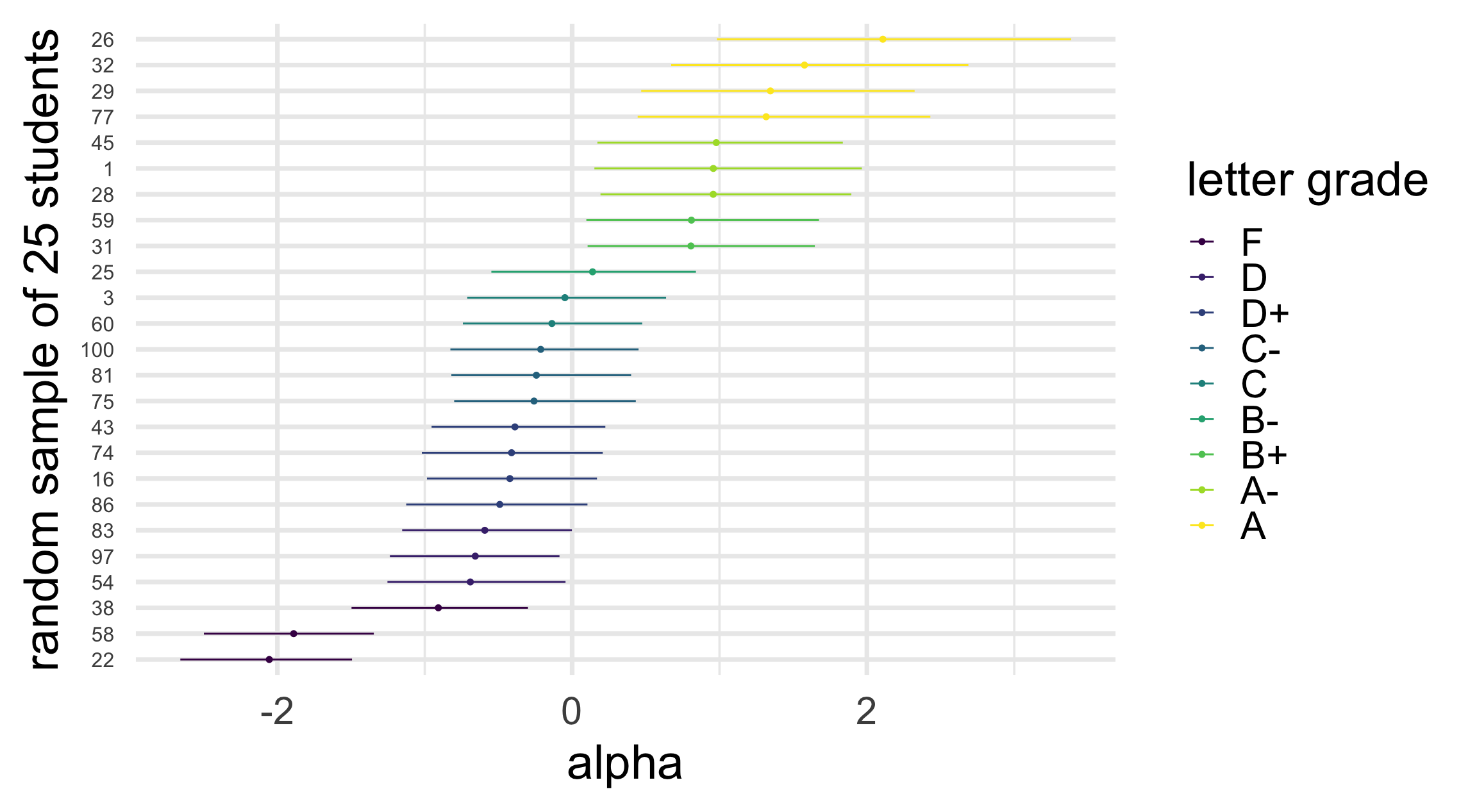

Using `spread_draws()` from {tidybayes}

spread_draws(fit, beta[question_id_num])

# A tibble: 275,000 × 5
# Groups:   question_id_num [55]
   question_id_num   beta .chain .iteration .draw
             <int>  <dbl>  <int>      <int> <int>
 1               1 -0.145      1          1     1
 2               1 -0.838      1          2     2
 3               1 -0.793      1          3     3
 4               1 -0.128      1          4     4
 5               1 -0.994      1          5     5
 6               1 -0.557      1          6     6
 7               1 -1.03       1          7     7
 8               1 -0.795      1          8     8
 9               1 -0.420      1          9     9
10               1 -0.658      1         10    10
# ℹ 274,990 more rows

Adding `median_qi()` from {tidybayes}

spread_draws(fit, beta[question_id_num]) |>
  median_qi()

# A tibble: 55 × 7
   question_id_num   beta  .lower .upper .width .point .interval
             <int>  <dbl>   <dbl>  <dbl>  <dbl> <chr>  <chr>    
 1               1 -0.652 -1.24   -0.108   0.95 median qi       
 2               2 -0.898 -1.53   -0.316   0.95 median qi       
 3               3 -0.140 -0.656   0.355   0.95 median qi       
 4               4 -0.255 -0.802   0.253   0.95 median qi       
 5               5 -0.135 -0.654   0.368   0.95 median qi       
 6               6  0.141 -0.351   0.627   0.95 median qi       
 7               7  0.493  0.0235  0.948   0.95 median qi       
 8               8 -0.808 -1.41   -0.273   0.95 median qi       
 9               9 -0.732 -1.31   -0.187   0.95 median qi       
10              10  0.451 -0.0280  0.909   0.95 median qi       
# ℹ 45 more rows

Now sort the questions

spread_draws(fit, beta[question_id_num]) |>
  median_qi() |>
  arrange(desc(beta))

# A tibble: 55 × 7
   question_id_num  beta .lower .upper .width .point .interval
             <int> <dbl>  <dbl>  <dbl>  <dbl> <chr>  <chr>    
 1              27 1.57   1.12    2.02   0.95 median qi       
 2              28 1.52   1.08    1.98   0.95 median qi       
 3              13 0.995  0.546   1.45   0.95 median qi       
 4              49 0.995  0.549   1.45   0.95 median qi       
 5              43 0.908  0.451   1.37   0.95 median qi       
 6              46 0.865  0.403   1.31   0.95 median qi       
 7              52 0.771  0.321   1.24   0.95 median qi       
 8              35 0.726  0.291   1.18   0.95 median qi       
 9              53 0.682  0.224   1.14   0.95 median qi       
10              44 0.584  0.127   1.05   0.95 median qi       
# ℹ 45 more rows

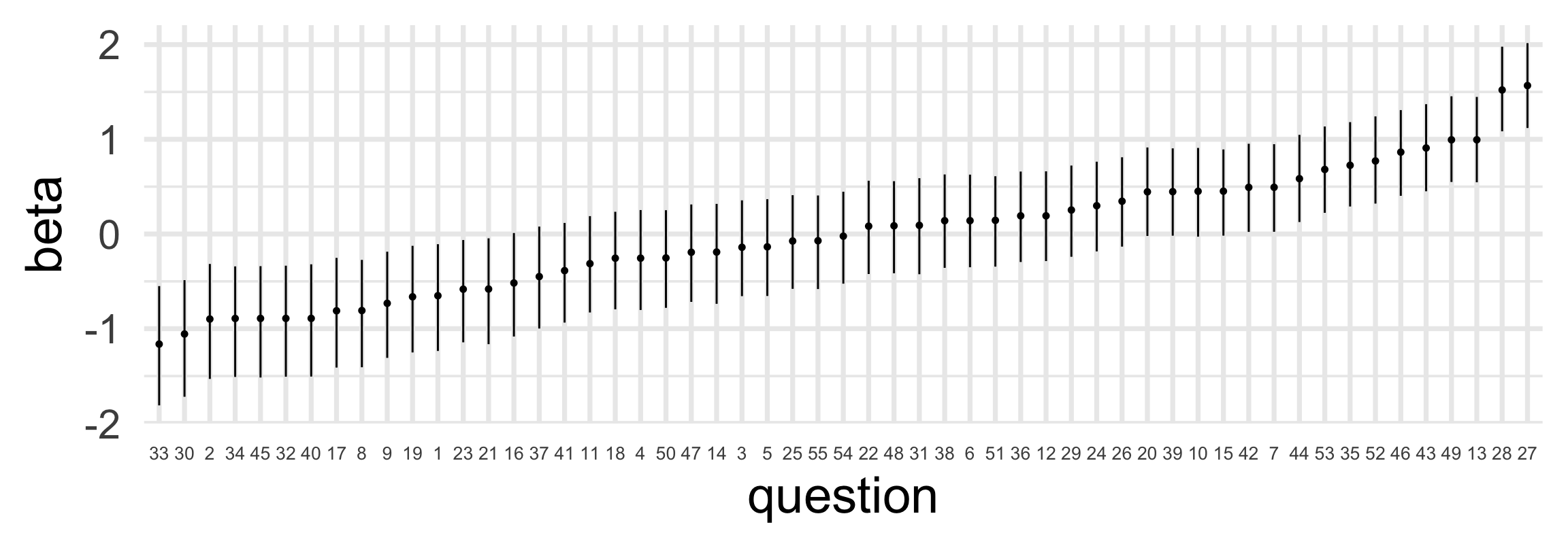
Plot the difficulties

Code

fit %>%
  spread_draws(beta[question_id_num]) %>%
  median_qi() %>%
  ggplot(aes(y = beta, ymin = .lower, ymax = .upper,
             x = reorder(question_id_num, beta))) +
  geom_pointinterval(linewidth = 0.5, size = 0.5) +
  labs(x = "question") +
  theme(axis.text.x = element_text(size = 10))

Fitting with `brm()`

f <- correct_answer ~ (1 | question_id_num) + (1 | student_id_num)
brm_fit <- brm(f, data = answers, family = bernoulli, chains = 10, cores = 10,
               iter = 1000, warmup = 500, backend = "cmdstanr")

The list of output from brm() includes a fit that is just the output from $sample() above. We can use this element if we want, but the parameters have less nice names.

print(brm_fit$fit)

Inference for Stan model: model_636ac9730bf7a0d98d68e8af455f14b9-202611030835-1-5c1928.
10 chains, each with iter=1000; warmup=500; thin=1; 
post-warmup draws per chain=500, total post-warmup draws=5000.

                                    mean se_mean    sd     2.5%      25%      50%
b_Intercept                         1.35    0.01  0.14     1.07     1.25     1.35
sd_question_id_num__Intercept       0.72    0.00  0.08     0.58     0.66     0.71
sd_student_id_num__Intercept        0.98    0.00  0.09     0.82     0.92     0.98
Intercept                           1.35    0.01  0.14     1.07     1.25     1.35
r_question_id_num[1,Intercept]      0.67    0.00  0.29     0.13     0.47     0.66
r_question_id_num[2,Intercept]      0.90    0.00  0.30     0.34     0.70     0.89
r_question_id_num[3,Intercept]      0.14    0.01  0.26    -0.34    -0.04     0.14
r_question_id_num[4,Intercept]      0.26    0.00  0.26    -0.25     0.09     0.26
r_question_id_num[5,Intercept]      0.14    0.01  0.26    -0.37    -0.04     0.14
r_question_id_num[6,Intercept]     -0.14    0.00  0.25    -0.62    -0.31    -0.15
r_question_id_num[7,Intercept]     -0.49    0.00  0.23    -0.95    -0.65    -0.50
r_question_id_num[8,Intercept]      0.82    0.00  0.31     0.25     0.61     0.81
r_question_id_num[9,Intercept]      0.74    0.00  0.29     0.17     0.54     0.73
r_question_id_num[10,Intercept]    -0.45    0.00  0.24    -0.90    -0.61    -0.45
r_question_id_num[11,Intercept]     0.32    0.00  0.27    -0.19     0.14     0.31
r_question_id_num[12,Intercept]    -0.20    0.00  0.25    -0.69    -0.37    -0.20
r_question_id_num[13,Intercept]    -1.00    0.00  0.23    -1.47    -1.16    -1.00
r_question_id_num[14,Intercept]     0.20    0.00  0.27    -0.31     0.01     0.19
r_question_id_num[15,Intercept]    -0.44    0.00  0.24    -0.90    -0.60    -0.45
r_question_id_num[16,Intercept]     0.52    0.00  0.27    -0.01     0.33     0.51
r_question_id_num[17,Intercept]     0.82    0.00  0.30     0.24     0.62     0.82
r_question_id_num[18,Intercept]     0.25    0.00  0.26    -0.26     0.07     0.25
r_question_id_num[19,Intercept]     0.66    0.00  0.29     0.11     0.46     0.66
r_question_id_num[20,Intercept]    -0.45    0.00  0.24    -0.90    -0.62    -0.45
r_question_id_num[21,Intercept]     0.59    0.00  0.28     0.05     0.40     0.58
r_question_id_num[22,Intercept]    -0.09    0.00  0.25    -0.57    -0.25    -0.09
r_question_id_num[23,Intercept]     0.60    0.00  0.28     0.06     0.40     0.59
r_question_id_num[24,Intercept]    -0.30    0.00  0.25    -0.78    -0.47    -0.30
r_question_id_num[25,Intercept]     0.08    0.00  0.25    -0.41    -0.09     0.08
r_question_id_num[26,Intercept]    -0.35    0.00  0.24    -0.83    -0.51    -0.35
r_question_id_num[27,Intercept]    -1.58    0.00  0.23    -2.04    -1.74    -1.58
r_question_id_num[28,Intercept]    -1.53    0.00  0.23    -1.99    -1.69    -1.53
r_question_id_num[29,Intercept]    -0.25    0.00  0.25    -0.73    -0.41    -0.25
r_question_id_num[30,Intercept]     1.07    0.00  0.32     0.46     0.85     1.06
r_question_id_num[31,Intercept]    -0.09    0.00  0.25    -0.57    -0.25    -0.09
r_question_id_num[32,Intercept]     0.90    0.01  0.30     0.34     0.69     0.89
r_question_id_num[33,Intercept]     1.17    0.01  0.33     0.57     0.95     1.16
r_question_id_num[34,Intercept]     0.91    0.00  0.31     0.34     0.69     0.90
r_question_id_num[35,Intercept]    -0.73    0.00  0.23    -1.20    -0.89    -0.74
r_question_id_num[36,Intercept]    -0.19    0.00  0.24    -0.66    -0.35    -0.20
r_question_id_num[37,Intercept]     0.45    0.00  0.27    -0.07     0.27     0.45
r_question_id_num[38,Intercept]    -0.14    0.00  0.24    -0.62    -0.31    -0.15
r_question_id_num[39,Intercept]    -0.45    0.00  0.24    -0.91    -0.61    -0.45
r_question_id_num[40,Intercept]     0.91    0.00  0.31     0.33     0.69     0.90
r_question_id_num[41,Intercept]     0.39    0.00  0.27    -0.14     0.20     0.39
r_question_id_num[42,Intercept]    -0.50    0.00  0.23    -0.97    -0.66    -0.51
r_question_id_num[43,Intercept]    -0.92    0.00  0.23    -1.36    -1.07    -0.91
r_question_id_num[44,Intercept]    -0.59    0.00  0.24    -1.06    -0.75    -0.59
r_question_id_num[45,Intercept]     0.90    0.00  0.30     0.34     0.69     0.90
r_question_id_num[46,Intercept]    -0.87    0.00  0.24    -1.33    -1.03    -0.87
r_question_id_num[47,Intercept]     0.20    0.00  0.26    -0.29     0.02     0.19
r_question_id_num[48,Intercept]    -0.09    0.00  0.26    -0.59    -0.26    -0.09
r_question_id_num[49,Intercept]    -1.00    0.00  0.23    -1.45    -1.16    -1.01
r_question_id_num[50,Intercept]     0.26    0.00  0.27    -0.25     0.08     0.25
r_question_id_num[51,Intercept]    -0.14    0.00  0.25    -0.62    -0.32    -0.14
r_question_id_num[52,Intercept]    -0.78    0.00  0.24    -1.24    -0.94    -0.78
r_question_id_num[53,Intercept]    -0.69    0.00  0.23    -1.14    -0.85    -0.69
r_question_id_num[54,Intercept]     0.02    0.00  0.25    -0.47    -0.15     0.02
r_question_id_num[55,Intercept]     0.08    0.00  0.26    -0.41    -0.10     0.07
r_student_id_num[1,Intercept]       0.98    0.01  0.41     0.22     0.69     0.96
r_student_id_num[2,Intercept]      -1.14    0.01  0.29    -1.72    -1.33    -1.14
r_student_id_num[3,Intercept]      -0.03    0.01  0.34    -0.68    -0.26    -0.04
r_student_id_num[4,Intercept]      -0.23    0.01  0.33    -0.87    -0.46    -0.24
r_student_id_num[5,Intercept]       1.59    0.01  0.51     0.66     1.25     1.57
r_student_id_num[6,Intercept]       0.29    0.01  0.36    -0.40     0.04     0.28
r_student_id_num[7,Intercept]       0.29    0.01  0.35    -0.36     0.05     0.29
r_student_id_num[8,Intercept]       0.06    0.01  0.34    -0.58    -0.18     0.06
r_student_id_num[9,Intercept]      -0.98    0.01  0.30    -1.57    -1.19    -0.99
r_student_id_num[10,Intercept]      0.17    0.01  0.35    -0.48    -0.07     0.17
r_student_id_num[11,Intercept]      0.53    0.01  0.37    -0.16     0.27     0.52
r_student_id_num[12,Intercept]     -0.75    0.01  0.30    -1.31    -0.95    -0.75
r_student_id_num[13,Intercept]     -0.14    0.01  0.33    -0.75    -0.36    -0.15
r_student_id_num[14,Intercept]      1.59    0.01  0.50     0.70     1.23     1.56
r_student_id_num[15,Intercept]      0.17    0.01  0.35    -0.50    -0.06     0.17
r_student_id_num[16,Intercept]     -0.41    0.01  0.30    -0.98    -0.62    -0.41
r_student_id_num[17,Intercept]     -0.75    0.01  0.30    -1.34    -0.95    -0.75
r_student_id_num[18,Intercept]      1.60    0.01  0.51     0.67     1.25     1.58
r_student_id_num[19,Intercept]      1.16    0.01  0.45     0.34     0.85     1.15
r_student_id_num[20,Intercept]      0.53    0.01  0.38    -0.20     0.28     0.52
r_student_id_num[21,Intercept]     -0.14    0.01  0.33    -0.77    -0.36    -0.14
r_student_id_num[22,Intercept]     -2.06    0.00  0.30    -2.67    -2.26    -2.05
r_student_id_num[23,Intercept]     -0.67    0.01  0.30    -1.26    -0.87    -0.67
r_student_id_num[24,Intercept]     -0.74    0.01  0.31    -1.34    -0.95    -0.75
r_student_id_num[25,Intercept]      0.18    0.01  0.35    -0.47    -0.06     0.16
r_student_id_num[26,Intercept]      2.16    0.01  0.60     1.08     1.73     2.12
r_student_id_num[27,Intercept]     -0.58    0.00  0.31    -1.18    -0.80    -0.59
r_student_id_num[28,Intercept]      0.98    0.01  0.41     0.20     0.70     0.96
r_student_id_num[29,Intercept]      1.37    0.01  0.48     0.49     1.03     1.35
r_student_id_num[30,Intercept]      0.98    0.01  0.42     0.20     0.69     0.97
r_student_id_num[31,Intercept]      0.82    0.01  0.40     0.07     0.54     0.80
r_student_id_num[32,Intercept]      1.58    0.01  0.51     0.64     1.21     1.56
r_student_id_num[33,Intercept]      0.99    0.01  0.42     0.19     0.71     0.97
r_student_id_num[34,Intercept]      0.81    0.01  0.40     0.05     0.53     0.79
r_student_id_num[35,Intercept]      1.36    0.01  0.47     0.50     1.04     1.35
r_student_id_num[36,Intercept]     -0.42    0.01  0.32    -1.02    -0.64    -0.42
r_student_id_num[37,Intercept]     -0.50    0.01  0.31    -1.09    -0.72    -0.50
r_student_id_num[38,Intercept]     -0.90    0.01  0.30    -1.47    -1.11    -0.91
r_student_id_num[39,Intercept]      0.54    0.01  0.38    -0.18     0.28     0.52
r_student_id_num[40,Intercept]     -0.50    0.01  0.31    -1.10    -0.70    -0.50
r_student_id_num[41,Intercept]     -1.36    0.01  0.29    -1.92    -1.57    -1.35
r_student_id_num[42,Intercept]      0.98    0.01  0.43     0.17     0.68     0.96
r_student_id_num[43,Intercept]     -0.42    0.01  0.31    -1.01    -0.62    -0.42
r_student_id_num[44,Intercept]      0.98    0.01  0.42     0.21     0.69     0.97
r_student_id_num[45,Intercept]      0.98    0.01  0.43     0.19     0.68     0.97
r_student_id_num[46,Intercept]      0.41    0.01  0.37    -0.26     0.15     0.40
r_student_id_num[47,Intercept]      0.41    0.01  0.37    -0.28     0.15     0.40
r_student_id_num[48,Intercept]     -0.05    0.01  0.33    -0.68    -0.27    -0.04
r_student_id_num[49,Intercept]     -1.06    0.01  0.29    -1.63    -1.26    -1.06
r_student_id_num[50,Intercept]     -1.22    0.01  0.29    -1.78    -1.41    -1.21
r_student_id_num[51,Intercept]     -0.23    0.01  0.33    -0.89    -0.45    -0.24
r_student_id_num[52,Intercept]     -0.03    0.01  0.33    -0.66    -0.26    -0.04
r_student_id_num[53,Intercept]     -1.14    0.01  0.30    -1.70    -1.34    -1.14
r_student_id_num[54,Intercept]     -0.67    0.01  0.30    -1.26    -0.87    -0.67
r_student_id_num[55,Intercept]      0.41    0.01  0.36    -0.27     0.16     0.39
r_student_id_num[56,Intercept]      0.28    0.01  0.36    -0.40     0.04     0.27
r_student_id_num[57,Intercept]      0.53    0.01  0.37    -0.16     0.29     0.52
r_student_id_num[58,Intercept]     -1.90    0.01  0.30    -2.49    -2.10    -1.90
r_student_id_num[59,Intercept]      0.82    0.01  0.41     0.06     0.54     0.80
r_student_id_num[60,Intercept]     -0.13    0.01  0.33    -0.78    -0.36    -0.14
r_student_id_num[61,Intercept]     -0.58    0.01  0.31    -1.17    -0.79    -0.59
r_student_id_num[62,Intercept]     -0.40    0.01  0.31    -1.00    -0.62    -0.40
r_student_id_num[63,Intercept]     -0.23    0.01  0.32    -0.85    -0.45    -0.24
r_student_id_num[64,Intercept]      0.18    0.01  0.34    -0.47    -0.06     0.17
r_student_id_num[65,Intercept]      1.61    0.01  0.52     0.69     1.24     1.58
r_student_id_num[66,Intercept]     -0.23    0.01  0.32    -0.85    -0.45    -0.23
r_student_id_num[67,Intercept]     -2.41    0.00  0.32    -3.03    -2.62    -2.41
r_student_id_num[68,Intercept]     -1.06    0.01  0.29    -1.62    -1.26    -1.06
r_student_id_num[69,Intercept]     -1.14    0.01  0.29    -1.70    -1.34    -1.14
r_student_id_num[70,Intercept]     -1.14    0.01  0.29    -1.68    -1.33    -1.14
r_student_id_num[71,Intercept]      0.41    0.01  0.36    -0.25     0.16     0.39
r_student_id_num[72,Intercept]     -0.33    0.01  0.31    -0.94    -0.54    -0.33
r_student_id_num[73,Intercept]      0.99    0.01  0.43     0.18     0.69     0.97
r_student_id_num[74,Intercept]     -0.41    0.01  0.32    -1.04    -0.62    -0.42
r_student_id_num[75,Intercept]     -0.23    0.01  0.32    -0.84    -0.45    -0.24
r_student_id_num[76,Intercept]     -0.24    0.01  0.32    -0.84    -0.46    -0.24
r_student_id_num[77,Intercept]      1.37    0.01  0.48     0.50     1.04     1.34
r_student_id_num[78,Intercept]     -1.29    0.01  0.29    -1.86    -1.48    -1.29
r_student_id_num[79,Intercept]      0.17    0.01  0.35    -0.49    -0.08     0.16
r_student_id_num[80,Intercept]     -0.24    0.01  0.31    -0.87    -0.44    -0.24
r_student_id_num[81,Intercept]     -0.23    0.01  0.32    -0.83    -0.45    -0.23
r_student_id_num[82,Intercept]      0.68    0.01  0.39    -0.07     0.40     0.66
r_student_id_num[83,Intercept]     -0.58    0.01  0.31    -1.18    -0.78    -0.57
r_student_id_num[84,Intercept]     -0.91    0.01  0.30    -1.49    -1.11    -0.91
r_student_id_num[85,Intercept]     -0.82    0.00  0.30    -1.41    -1.04    -0.83
r_student_id_num[86,Intercept]     -0.50    0.01  0.31    -1.10    -0.71    -0.51
r_student_id_num[87,Intercept]      1.36    0.01  0.47     0.49     1.03     1.34
r_student_id_num[88,Intercept]      0.28    0.01  0.35    -0.40     0.04     0.28
r_student_id_num[89,Intercept]      0.06    0.01  0.34    -0.59    -0.17     0.05
r_student_id_num[90,Intercept]      0.40    0.01  0.36    -0.28     0.15     0.39
r_student_id_num[91,Intercept]      1.85    0.01  0.56     0.85     1.47     1.82
r_student_id_num[92,Intercept]     -0.75    0.01  0.30    -1.32    -0.96    -0.75
r_student_id_num[93,Intercept]      0.53    0.01  0.37    -0.17     0.27     0.52
r_student_id_num[94,Intercept]     -0.04    0.01  0.33    -0.65    -0.27    -0.05
r_student_id_num[95,Intercept]     -0.22    0.01  0.32    -0.84    -0.44    -0.23
r_student_id_num[96,Intercept]     -1.67    0.00  0.29    -2.25    -1.87    -1.67
r_student_id_num[97,Intercept]     -0.67    0.01  0.30    -1.25    -0.87    -0.67
r_student_id_num[98,Intercept]     -0.14    0.01  0.33    -0.76    -0.36    -0.14
r_student_id_num[99,Intercept]      0.06    0.01  0.34    -0.59    -0.17     0.05
r_student_id_num[100,Intercept]    -0.23    0.01  0.32    -0.85    -0.45    -0.23
lprior                             -4.71    0.00  0.04    -4.80    -4.74    -4.70
lp__                            -2822.19    0.45 12.85 -2848.06 -2830.77 -2821.63
                                     75%    97.5% n_eff Rhat
b_Intercept                         1.44     1.63   581 1.02
sd_question_id_num__Intercept       0.77     0.90   968 1.01
sd_student_id_num__Intercept        1.04     1.16   911 1.01
Intercept                           1.44     1.63   581 1.02
r_question_id_num[1,Intercept]      0.86     1.26  3827 1.00
r_question_id_num[2,Intercept]      1.10     1.52  4262 1.00
r_question_id_num[3,Intercept]      0.31     0.66  2547 1.00
r_question_id_num[4,Intercept]      0.45     0.78  2811 1.00
r_question_id_num[5,Intercept]      0.32     0.66  2741 1.00
r_question_id_num[6,Intercept]      0.03     0.35  3120 1.00
r_question_id_num[7,Intercept]     -0.33    -0.03  2883 1.00
r_question_id_num[8,Intercept]      1.02     1.46  3917 1.00
r_question_id_num[9,Intercept]      0.93     1.32  3896 1.00
r_question_id_num[10,Intercept]    -0.29     0.02  2898 1.00
r_question_id_num[11,Intercept]     0.50     0.85  3572 1.00
r_question_id_num[12,Intercept]    -0.03     0.29  3039 1.00
r_question_id_num[13,Intercept]    -0.85    -0.55  3071 1.00
r_question_id_num[14,Intercept]     0.38     0.74  3534 1.00
r_question_id_num[15,Intercept]    -0.28     0.02  2960 1.00
r_question_id_num[16,Intercept]     0.70     1.06  3761 1.00
r_question_id_num[17,Intercept]     1.02     1.44  3695 1.00
r_question_id_num[18,Intercept]     0.43     0.77  3635 1.00
r_question_id_num[19,Intercept]     0.85     1.24  4147 1.00
r_question_id_num[20,Intercept]    -0.29     0.02  2995 1.00
r_question_id_num[21,Intercept]     0.77     1.16  3958 1.00
r_question_id_num[22,Intercept]     0.08     0.41  2617 1.00
r_question_id_num[23,Intercept]     0.78     1.16  3578 1.00
r_question_id_num[24,Intercept]    -0.13     0.17  2925 1.00
r_question_id_num[25,Intercept]     0.24     0.58  3141 1.00
r_question_id_num[26,Intercept]    -0.19     0.13  2761 1.00
r_question_id_num[27,Intercept]    -1.42    -1.13  3373 1.00
r_question_id_num[28,Intercept]    -1.37    -1.09  2958 1.00
r_question_id_num[29,Intercept]    -0.09     0.25  2756 1.00
r_question_id_num[30,Intercept]     1.29     1.71  4103 1.00
r_question_id_num[31,Intercept]     0.08     0.41  3109 1.00
r_question_id_num[32,Intercept]     1.10     1.52  3277 1.00
r_question_id_num[33,Intercept]     1.38     1.86  3509 1.00
r_question_id_num[34,Intercept]     1.11     1.54  4040 1.00
r_question_id_num[35,Intercept]    -0.57    -0.27  3028 1.00
r_question_id_num[36,Intercept]    -0.03     0.30  3220 1.00
r_question_id_num[37,Intercept]     0.64     0.98  3417 1.00
r_question_id_num[38,Intercept]     0.02     0.34  2827 1.00
r_question_id_num[39,Intercept]    -0.29     0.03  2863 1.00
r_question_id_num[40,Intercept]     1.11     1.54  4163 1.00
r_question_id_num[41,Intercept]     0.57     0.92  3328 1.00
r_question_id_num[42,Intercept]    -0.35    -0.04  2470 1.00
r_question_id_num[43,Intercept]    -0.76    -0.46  3082 1.00
r_question_id_num[44,Intercept]    -0.43    -0.13  2725 1.00
r_question_id_num[45,Intercept]     1.10     1.52  4078 1.00
r_question_id_num[46,Intercept]    -0.71    -0.40  2549 1.00
r_question_id_num[47,Intercept]     0.37     0.73  3699 1.00
r_question_id_num[48,Intercept]     0.09     0.41  3082 1.00
r_question_id_num[49,Intercept]    -0.85    -0.54  2974 1.00
r_question_id_num[50,Intercept]     0.43     0.82  3066 1.00
r_question_id_num[51,Intercept]     0.02     0.36  2658 1.00
r_question_id_num[52,Intercept]    -0.62    -0.31  2962 1.00
r_question_id_num[53,Intercept]    -0.53    -0.24  2659 1.00
r_question_id_num[54,Intercept]     0.19     0.54  2977 1.00
r_question_id_num[55,Intercept]     0.25     0.59  3154 1.00
r_student_id_num[1,Intercept]       1.24     1.84  4580 1.00
r_student_id_num[2,Intercept]      -0.94    -0.59  3135 1.00
r_student_id_num[3,Intercept]       0.19     0.64  2997 1.00
r_student_id_num[4,Intercept]      -0.01     0.42  3624 1.00
r_student_id_num[5,Intercept]       1.90     2.68  4522 1.00
r_student_id_num[6,Intercept]       0.52     1.03  4290 1.00
r_student_id_num[7,Intercept]       0.51     1.01  3814 1.00
r_student_id_num[8,Intercept]       0.29     0.77  3360 1.00
r_student_id_num[9,Intercept]      -0.78    -0.40  3125 1.00
r_student_id_num[10,Intercept]      0.40     0.88  3644 1.00
r_student_id_num[11,Intercept]      0.78     1.26  3887 1.00
r_student_id_num[12,Intercept]     -0.54    -0.15  3237 1.00
r_student_id_num[13,Intercept]      0.08     0.52  3671 1.00
r_student_id_num[14,Intercept]      1.92     2.64  5126 1.00
r_student_id_num[15,Intercept]      0.40     0.87  3585 1.00
r_student_id_num[16,Intercept]     -0.20     0.21  2860 1.00
r_student_id_num[17,Intercept]     -0.55    -0.13  3137 1.00
r_student_id_num[18,Intercept]      1.93     2.66  4084 1.00
r_student_id_num[19,Intercept]      1.45     2.08  3903 1.00
r_student_id_num[20,Intercept]      0.78     1.30  3138 1.00
r_student_id_num[21,Intercept]      0.07     0.53  3631 1.00
r_student_id_num[22,Intercept]     -1.86    -1.46  3905 1.00
r_student_id_num[23,Intercept]     -0.46    -0.08  3404 1.00
r_student_id_num[24,Intercept]     -0.55    -0.13  2938 1.00
r_student_id_num[25,Intercept]      0.40     0.90  3747 1.00
r_student_id_num[26,Intercept]      2.53     3.46  4567 1.00
r_student_id_num[27,Intercept]     -0.37     0.06  4107 1.00
r_student_id_num[28,Intercept]      1.24     1.85  4919 1.00
r_student_id_num[29,Intercept]      1.68     2.35  4931 1.00
r_student_id_num[30,Intercept]      1.26     1.84  3639 1.00
r_student_id_num[31,Intercept]      1.09     1.62  4292 1.00
r_student_id_num[32,Intercept]      1.92     2.67  3804 1.00
r_student_id_num[33,Intercept]      1.25     1.85  4770 1.00
r_student_id_num[34,Intercept]      1.08     1.64  3912 1.00
r_student_id_num[35,Intercept]      1.66     2.32  5014 1.00
r_student_id_num[36,Intercept]     -0.20     0.23  3176 1.00
r_student_id_num[37,Intercept]     -0.30     0.13  3278 1.00
r_student_id_num[38,Intercept]     -0.71    -0.32  2886 1.00
r_student_id_num[39,Intercept]      0.79     1.30  4452 1.00
r_student_id_num[40,Intercept]     -0.29     0.11  3656 1.00
r_student_id_num[41,Intercept]     -1.16    -0.81  3056 1.00
r_student_id_num[42,Intercept]      1.25     1.88  4668 1.00
r_student_id_num[43,Intercept]     -0.21     0.19  3665 1.00
r_student_id_num[44,Intercept]      1.25     1.86  3896 1.00
r_student_id_num[45,Intercept]      1.26     1.84  4775 1.00
r_student_id_num[46,Intercept]      0.66     1.17  4182 1.00
r_student_id_num[47,Intercept]      0.65     1.14  3804 1.00
r_student_id_num[48,Intercept]      0.18     0.58  4192 1.00
r_student_id_num[49,Intercept]     -0.87    -0.49  3128 1.00
r_student_id_num[50,Intercept]     -1.02    -0.64  3148 1.00
r_student_id_num[51,Intercept]     -0.01     0.43  3730 1.00
r_student_id_num[52,Intercept]      0.18     0.62  3767 1.00
r_student_id_num[53,Intercept]     -0.94    -0.54  3004 1.00
r_student_id_num[54,Intercept]     -0.47    -0.05  3295 1.00
r_student_id_num[55,Intercept]      0.64     1.16  3822 1.00
r_student_id_num[56,Intercept]      0.52     1.03  3411 1.00
r_student_id_num[57,Intercept]      0.76     1.28  3744 1.00
r_student_id_num[58,Intercept]     -1.70    -1.32  3479 1.00
r_student_id_num[59,Intercept]      1.08     1.69  3198 1.00
r_student_id_num[60,Intercept]      0.09     0.53  3528 1.00
r_student_id_num[61,Intercept]     -0.37     0.04  3773 1.00
r_student_id_num[62,Intercept]     -0.19     0.21  3375 1.00
r_student_id_num[63,Intercept]     -0.01     0.41  3755 1.00
r_student_id_num[64,Intercept]      0.40     0.88  3647 1.00
r_student_id_num[65,Intercept]      1.94     2.72  4523 1.00
r_student_id_num[66,Intercept]     -0.02     0.41  3710 1.00
r_student_id_num[67,Intercept]     -2.19    -1.78  4607 1.00
r_student_id_num[68,Intercept]     -0.87    -0.47  3120 1.00
r_student_id_num[69,Intercept]     -0.95    -0.58  2630 1.00
r_student_id_num[70,Intercept]     -0.94    -0.57  2777 1.00
r_student_id_num[71,Intercept]      0.64     1.16  4110 1.00
r_student_id_num[72,Intercept]     -0.12     0.30  3436 1.00
r_student_id_num[73,Intercept]      1.27     1.89  4853 1.00
r_student_id_num[74,Intercept]     -0.20     0.22  3638 1.00
r_student_id_num[75,Intercept]     -0.03     0.40  3495 1.00
r_student_id_num[76,Intercept]     -0.01     0.40  2747 1.00
r_student_id_num[77,Intercept]      1.67     2.40  4290 1.00
r_student_id_num[78,Intercept]     -1.09    -0.73  2907 1.00
r_student_id_num[79,Intercept]      0.40     0.86  3591 1.00
r_student_id_num[80,Intercept]     -0.04     0.40  3268 1.00
r_student_id_num[81,Intercept]     -0.01     0.41  3129 1.00
r_student_id_num[82,Intercept]      0.94     1.49  3561 1.00
r_student_id_num[83,Intercept]     -0.37     0.02  3313 1.00
r_student_id_num[84,Intercept]     -0.70    -0.31  3501 1.00
r_student_id_num[85,Intercept]     -0.62    -0.22  3670 1.00
r_student_id_num[86,Intercept]     -0.29     0.12  2815 1.00
r_student_id_num[87,Intercept]      1.66     2.34  5651 1.00
r_student_id_num[88,Intercept]      0.52     0.99  3812 1.00
r_student_id_num[89,Intercept]      0.28     0.74  3426 1.00
r_student_id_num[90,Intercept]      0.64     1.12  4335 1.00
r_student_id_num[91,Intercept]      2.21     3.06  5019 1.00
r_student_id_num[92,Intercept]     -0.54    -0.17  3055 1.00
r_student_id_num[93,Intercept]      0.78     1.28  3687 1.00
r_student_id_num[94,Intercept]      0.17     0.61  3780 1.00
r_student_id_num[95,Intercept]     -0.01     0.44  3447 1.00
r_student_id_num[96,Intercept]     -1.47    -1.10  3467 1.00
r_student_id_num[97,Intercept]     -0.46    -0.07  3050 1.00
r_student_id_num[98,Intercept]      0.09     0.53  2450 1.00
r_student_id_num[99,Intercept]      0.27     0.76  3444 1.00
r_student_id_num[100,Intercept]    -0.02     0.42  3311 1.00
lprior                             -4.68    -4.63   819 1.01
lp__                            -2813.30 -2798.58   825 1.01

Samples were drawn using NUTS(diag_e) at Tue Nov 03 08:35:29 2026.
For each parameter, n_eff is a crude measure of effective sample size,
and Rhat is the potential scale reduction factor on split chains (at 
convergence, Rhat=1).

We can use the {tidybayes} functions on the `brm()` output

# brm()'s "r_question_id_num" plays the role of our "beta"
spread_draws(brm_fit, r_question_id_num[question_id_num, ]) |>
  median_qi() |>
  arrange(desc(-r_question_id_num))

# A tibble: 55 × 7
   question_id_num r_question_id_num .lower .upper .width .point .interval
             <int>             <dbl>  <dbl>  <dbl>  <dbl> <chr>  <chr>    
 1              27            -1.58   -2.04 -1.13    0.95 median qi       
 2              28            -1.53   -1.99 -1.09    0.95 median qi       
 3              49            -1.01   -1.45 -0.537   0.95 median qi       
 4              13            -1.00   -1.47 -0.549   0.95 median qi       
 5              43            -0.914  -1.36 -0.465   0.95 median qi       
 6              46            -0.871  -1.33 -0.402   0.95 median qi       
 7              52            -0.778  -1.24 -0.309   0.95 median qi       
 8              35            -0.736  -1.20 -0.270   0.95 median qi       
 9              53            -0.690  -1.14 -0.237   0.95 median qi       
10              44            -0.591  -1.06 -0.127   0.95 median qi       
# ℹ 45 more rows

Notice anything different?

And {marginaleffects}!

p <- predictions(brm_fit)
ggplot(p, aes(y = estimate, x = reorder(question_id_num, estimate))) +
  geom_point(alpha = 0.2) +
  geom_line(aes(group = student_id_num), alpha = 0.2) +
  labs(x = "question") +
  theme(axis.text.x = element_text(size = 10))

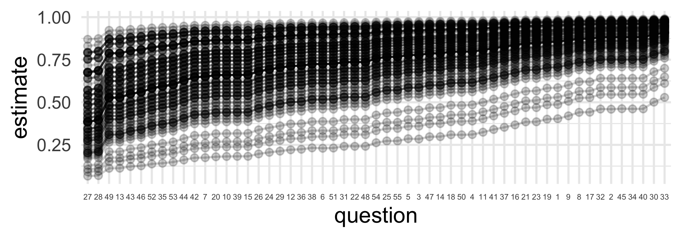
Fitting with `glmer()`

# fit model
f <- correct_answer ~ (1 | question_id_num) + (1 | student_id_num)
lmer_fit <- glmer(f, data = answers, family = binomial)

# grab "difficulties"
ranef(lmer_fit)$question_id_num |>
  as_tibble(rownames = "question_id_num") |>
  rename(beta = "(Intercept)") |>
  arrange(beta)

# A tibble: 55 × 2
   question_id_num   beta
   <chr>            <dbl>
 1 27              -1.56 
 2 28              -1.51 
 3 13              -1.00 
 4 49              -1.00 
 5 43              -0.916
 6 46              -0.873
 7 52              -0.785
 8 35              -0.740
 9 53              -0.695
10 44              -0.604
# ℹ 45 more rows

And more {marginaleffects}!

p <- predictions(lmer_fit)
ggplot(p, aes(y = estimate, x = reorder(question_id_num, estimate))) +
  geom_point(alpha = 0.2) +
  geom_line(aes(group = student_id_num), alpha = 0.2) +
  labs(x = "question") +
  theme(axis.text.x = element_text(size = 10))

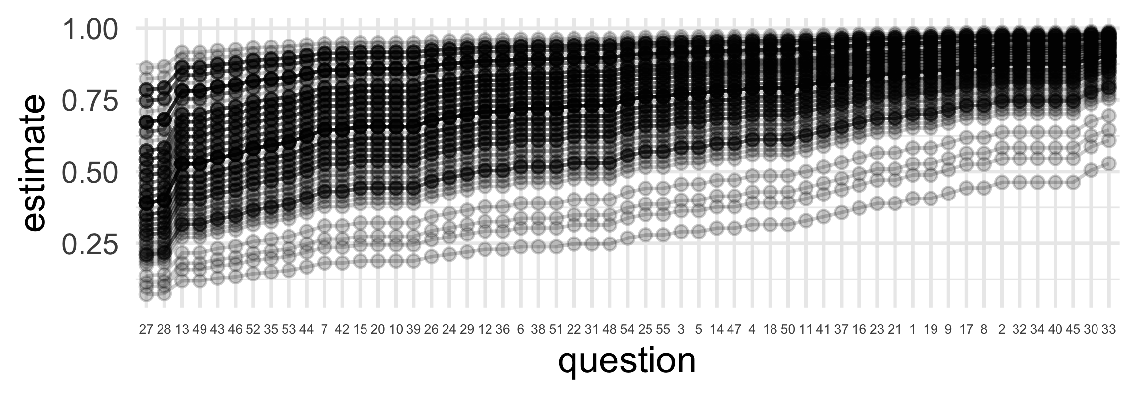
What if no partial pooling?

# fit model
f <- correct_answer ~ factor(question_id_num) + factor(student_id_num)
glm_fit <- glm(f, data = answers, family = binomial)

# marginaleffects
p1 <- predictions(glm_fit)
ggplot(p1, aes(y = estimate, x = reorder(question_id_num, estimate))) +
  geom_point(alpha = 0.2) +
  geom_line(aes(group = student_id_num), alpha = 0.2) +
  labs(x = "question") +
  theme(axis.text.x = element_text(size = 10))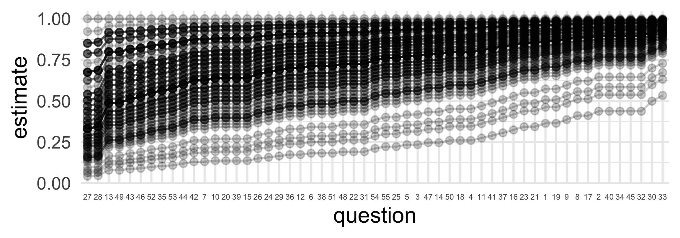

A plot of the partial pooling

Code

comb <- bind_rows(
  mutate(p, model = "glmer"),
  mutate(p1, model = "glm")) |>
mutate(question_id_num = reorder(factor(question_id_num), estimate))

ggplot(comb, aes(x = estimate, y = model)) +
  geom_point(alpha = 0.2) +
  geom_line(aes(group = rowid), alpha = 0.2) +
  facet_wrap(vars(question_id_num)) +
  theme_minimal(base_size = 12)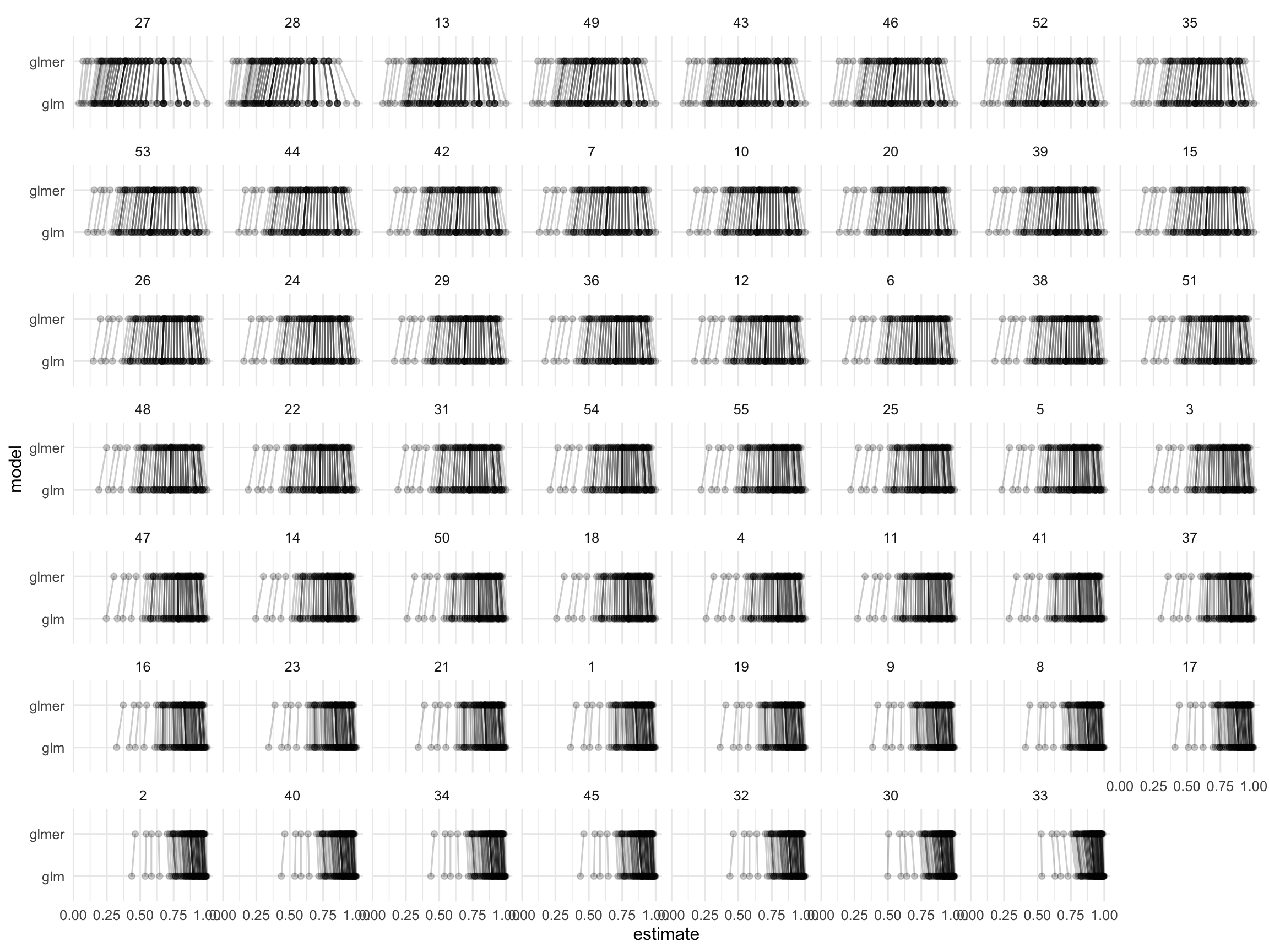

What if we gave each student 5 random questions?

If we give each student 5 random questions, this is really unfair! Some students will get hard questions. Other students will get easy questions.
BUT! We can use an IRT model to estimate the difficulty of each question and the ability of each student.
Even if the students don’t answer the same questions, we can put them on the same scale.
This won’t work super-great, each student answers only 5 questions and each question is asked only about 9 times. But it will help a little!

set.seed(1234)
random <- answers |>
  group_by(student_id_num) |>
  slice_sample(n = 5) %>%
  ungroup() %>%
  glimpse()

Rows: 500
Columns: 3
$ student_id_num  <dbl> 1, 1, 1, 1, 1, 2, 2, 2, 2, 2, 3, 3, 3, 3, 3, 4, 4, 4, 4, 4, 5, 5…
$ question_id_num <dbl> 28, 16, 22, 37, 44, 47, 9, 5, 38, 16, 4, 34, 39, 22, 26, 6, 15, …
$ correct_answer  <dbl> 1, 1, 1, 1, 0, 1, 0, 1, 1, 0, 1, 1, 1, 1, 1, 1, 1, 1, 0, 1, 1, 1…

Code

full_results <- answers |>
  group_by(student_id_num) |>
  summarize(score_on_full_exam = mean(correct_answer))

random_results <- random %>%
  group_by(student_id_num) |>
  summarize(score_on_random5_exam = mean(correct_answer))

comb <- full_results |>
  left_join(random_results)

print(comb)

# A tibble: 100 × 3
   student_id_num score_on_full_exam score_on_random5_exam
            <dbl>              <dbl>                 <dbl>
 1              1              0.909                   0.8
 2              2              0.527                   0.6
 3              3              0.764                   1  
 4              4              0.727                   0.8
 5              5              0.964                   1  
 6              6              0.818                   0.8
 7              7              0.818                   1  
 8              8              0.782                   1  
 9              9              0.564                   0.4
10             10              0.8                     0.8
# ℹ 90 more rows

# make a data frame with all observed and unobserved combos
# - each student *could have* been asked 55 questions; 50 answers are missing
all <- crossing(student_id_num = random$student_id_num,
                question_id_num = random$question_id_num) |>
  glimpse()

Rows: 5,500
Columns: 2
$ student_id_num  <dbl> 1, 1, 1, 1, 1, 1, 1, 1, 1, 1, 1, 1, 1, 1, 1, 1, 1, 1, 1, 1, 1, 1…
$ question_id_num <dbl> 1, 2, 3, 4, 5, 6, 7, 8, 9, 10, 11, 12, 13, 14, 15, 16, 17, 18, 1…

# fit irt model to observed answer
f <- correct_answer ~ (1 | question_id_num) + (1 | student_id_num)
random_lmer_fit <- glmer(f, data = random, family = binomial)

# fill in "answers" to the unanswered questions
modeled_answers <- all %>%
  mutate(pred = predict(random_lmer_fit, newdata = ., type = "response")) |>
  left_join(random) |>
  mutate(filled_correct_answer = case_when(is.na(correct_answer) ~ pred,
                                           TRUE ~ correct_answer)) |>
  glimpse()

Rows: 5,500
Columns: 5
$ student_id_num        <dbl> 1, 1, 1, 1, 1, 1, 1, 1, 1, 1, 1, 1, 1, 1, 1, 1, 1, 1, 1, 1…
$ question_id_num       <dbl> 1, 2, 3, 4, 5, 6, 7, 8, 9, 10, 11, 12, 13, 14, 15, 16, 17,…
$ pred                  <dbl> 0.757, 0.792, 0.837, 0.830, 0.797, 0.706, 0.707, 0.823, 0.…
$ correct_answer        <dbl> NA, NA, NA, NA, NA, NA, NA, NA, NA, NA, NA, NA, NA, NA, NA…
$ filled_correct_answer <dbl> 0.757, 0.792, 0.837, 0.830, 0.797, 0.706, 0.707, 0.823, 0.…

# compute scores
modeled_results <- modeled_answers |>
  group_by(student_id_num) |>
  summarize(modeled_score_on_random5_exam = mean(filled_correct_answer)) |>
  glimpse()

Rows: 100
Columns: 2
$ student_id_num                <dbl> 1, 2, 3, 4, 5, 6, 7, 8, 9, 10, 11, 12, 13, 14, 15,…
$ modeled_score_on_random5_exam <dbl> 0.773, 0.673, 0.851, 0.788, 0.838, 0.768, 0.846, 0…

comb <- full_results |>
  left_join(random_results) |>
  left_join(modeled_results) |>
  mutate(score_error = score_on_random5_exam - score_on_full_exam,
         modeled_score_error = modeled_score_on_random5_exam - score_on_full_exam) |>
  glimpse()

Rows: 100
Columns: 6
$ student_id_num                <dbl> 1, 2, 3, 4, 5, 6, 7, 8, 9, 10, 11, 12, 13, 14, 15,…
$ score_on_full_exam            <dbl> 0.909, 0.527, 0.764, 0.727, 0.964, 0.818, 0.818, 0…
$ score_on_random5_exam         <dbl> 0.8, 0.6, 1.0, 0.8, 1.0, 0.8, 1.0, 1.0, 0.4, 0.8, …
$ modeled_score_on_random5_exam <dbl> 0.773, 0.673, 0.851, 0.788, 0.838, 0.768, 0.846, 0…
$ score_error                   <dbl> -0.1091, 0.0727, 0.2364, 0.0727, 0.0364, -0.0182, …
$ modeled_score_error           <dbl> -0.13642, 0.14599, 0.08777, 0.06033, -0.12518, -0.…

Modeling reduces median abs. error by about 30%.

median(abs(comb$score_error))

[1] 0.109

median(abs(comb$modeled_score_error))

[1] 0.0762

median(abs(comb$modeled_score_error))/median(abs(comb$score_error)) - 1

[1] -0.302

Code

gg1 <- ggplot(comb, aes(x = score_on_full_exam, y = score_on_random5_exam)) +
  geom_jitter(height = 0.01, width = 0.01, alpha = 0.8, shape = 21) +
  geom_abline(intercept = 0, slope = 1)

gg2 <- ggplot(comb, aes(x = score_on_full_exam, y = modeled_score_on_random5_exam)) +
  geom_jitter(height = 0.01, width = 0.01, alpha = 0.8, shape = 21) +
  geom_abline(intercept = 0, slope = 1)

gg1 + gg2 &
  scale_y_continuous(limits = c(0, 1))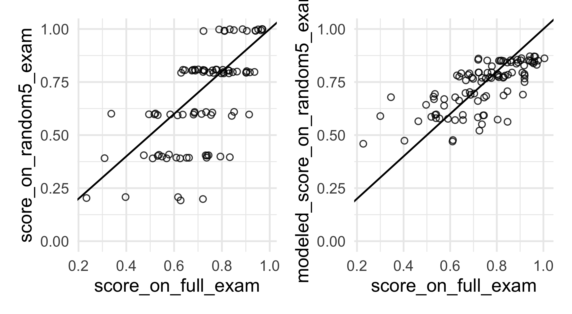

If you knew you were the worst student in the class, what method would you want the instructor to use? Best? Median?
Why does this happen?!? Is it good?

2-PL model

Indices

Answers: $n = 1, \dots, N$. ($N = 55 \times 100 = 5{,}500$ in our data.)
Students: $j = 1, \dots, J$. ($J = 100$ in our data.)
Questions: $k = 1, \dots, K$. ($K = 55$ in our data.)

Outcome: $y_{n} \in \{0, 1\}$ indicates whether the $n$th answer is correct.

\[ y_n \sim \text{Bernoulli}(\pi_n) \\ \pi_n = \operatorname{logit}^{-1} \left( \gamma_{k[n]} \left( \alpha_{j[n]} - \beta_{k[n]} \right) \right). \]

Parameters

$\pi_n$: the probability that answer $n$ is correct
$\alpha_{j[n]}$: the ability of student $j$ [who is giving the $n$th answer]
- Higher $\alpha_j$ ⇒ more likely to answer correctly; more knowledgeable student
$\beta_{k[n]}$: the difficulty of question $k$ [which is associated with the $n$th answer]
- Higher $\beta_k$ ⇒ less likely to answer correctly; harder item
$\gamma_{k[n]}$: the discrimination of question $k$
- Larger $\gamma_k$ ⇒ steeper item response curve; item better differentiates high- vs low-ability students

Exercise

Fit a 2-PL model to these data.

Identifiability in the 2-PL Model

Original

student $j$	question $k$	$\alpha_j$	$\gamma_k$	$\beta_k$	$\pi_{jk}$
1	1	0.5	1.0	-1.0	0.818
1	2	0.5	1.0	0.0	0.622
1	3	0.5	1.0	1.0	0.378
2	1	1.0	1.0	-1.0	0.881
2	2	1.0	1.0	0.0	0.731
2	3	1.0	1.0	1.0	0.500
3	1	1.5	1.0	-1.0	0.924
3	2	1.5	1.0	0.0	0.818
3	3	1.5	1.0	1.0	0.622

New Parameters, Same Probabilities

Transformation: $\alpha_j'=-2\,\alpha_j,\quad \beta_k'=-2\,\beta_k,\quad \gamma_k'=-\tfrac{1}{2}\,\gamma_k$

student $j$	question $k$	$\alpha_j'$	$\gamma_k'$	$\beta_k'$	$\pi_{jk}$
1	1	-1.0	-0.5	2.0	0.818
1	2	-1.0	-0.5	0.0	0.622
1	3	-1.0	-0.5	-2.0	0.378
2	1	-2.0	-0.5	2.0	0.881
2	2	-2.0	-0.5	0.0	0.731
2	3	-2.0	-0.5	-2.0	0.500
3	1	-3.0	-0.5	2.0	0.924
3	2	-3.0	-0.5	0.0	0.818
3	3	-3.0	-0.5	-2.0	0.622

Note

Key Idea:
Flipping the sign and scale of the latent ability (and compensating in the item and discrimination) parameters leaves the predicted probabilities $\pi_{jk}$ identical.

$\Rightarrow$ The 2-PL model is invariant to linear transformations of the latent ability scale:

\[ \alpha_j' = c(\alpha_j - d), \quad \gamma_k' = \frac{\gamma_k}{c}, \quad \beta_k' = c(\beta_k - d). \]

To identify the model, we fix:

Location: $E[\alpha_j]=0$
Scale: $\operatorname{Var}[\alpha_j]=1$
Direction: $\gamma_k > 0$

We could also allow $\gamma_k$ to be negative or positive and instead fix the sign of one of the $\alpha_j$.

IRT

IRT

The answers data

Grades on the exam

Rasch / 1-PL model

Hierarchical Model

Priors

Stan model

Set up data for Stan

What do these data look like?

A trick

Fit Stan model using {cmdstanr}

Print the fit

Using spread_draws() from {tidybayes}

Adding median_qi() from {tidybayes}

Plot the abilities for 25 random students

Using spread_draws() from {tidybayes}

Adding median_qi() from {tidybayes}

Now sort the questions

Plot the difficulties

Fitting with brm()

We can use the {tidybayes} functions on the brm() output

And {marginaleffects}!

Fitting with glmer()

And more {marginaleffects}!

What if no partial pooling?

A plot of the partial pooling

What if we gave each student 5 random questions?

2-PL model

Exercise

Identifiability in the 2-PL Model

Original

New Parameters, Same Probabilities

The `answers` data

Print the `fit`

Using `spread_draws()` from {tidybayes}

Adding `median_qi()` from {tidybayes}

Using `spread_draws()` from {tidybayes}

Adding `median_qi()` from {tidybayes}

Fitting with `brm()`

We can use the {tidybayes} functions on the `brm()` output

Fitting with `glmer()`