# generally useful packages
library(tidyverse)
library(marginaleffects)
library(modelsummary)
library(ggrepel)

# for fitting hierarchical models
library(lme4)
library(brms)  # see also rstanarm::stan_lmer()
library(rstan)

# for post-processing simulations
library(tidybayes)

# handle future conflicts
# - MASS v. dplyr for filter()
conflicted::conflict_prefer("filter", "dplyr")
# - MASS v. dplyr for select()
conflicted::conflict_prefer("select", "dplyr")
Ideal Points
Plot 1
Code
sc_summary <- sc |>
  group_by(justice, appointed_by) |>
  summarize(prop_cons_votes = mean(cons_vote, na.rm = TRUE)) |>
  ungroup() |>
  mutate(justice = reorder(justice, prop_cons_votes)) |>
  arrange(prop_cons_votes)

ggplot(sc_summary, aes(x = justice, y = prop_cons_votes)) +
  geom_col(width = 0.5) +
  geom_label(aes(label = scales::percent(prop_cons_votes, accuracy = 1)), hjust = 1.2) +
  coord_flip()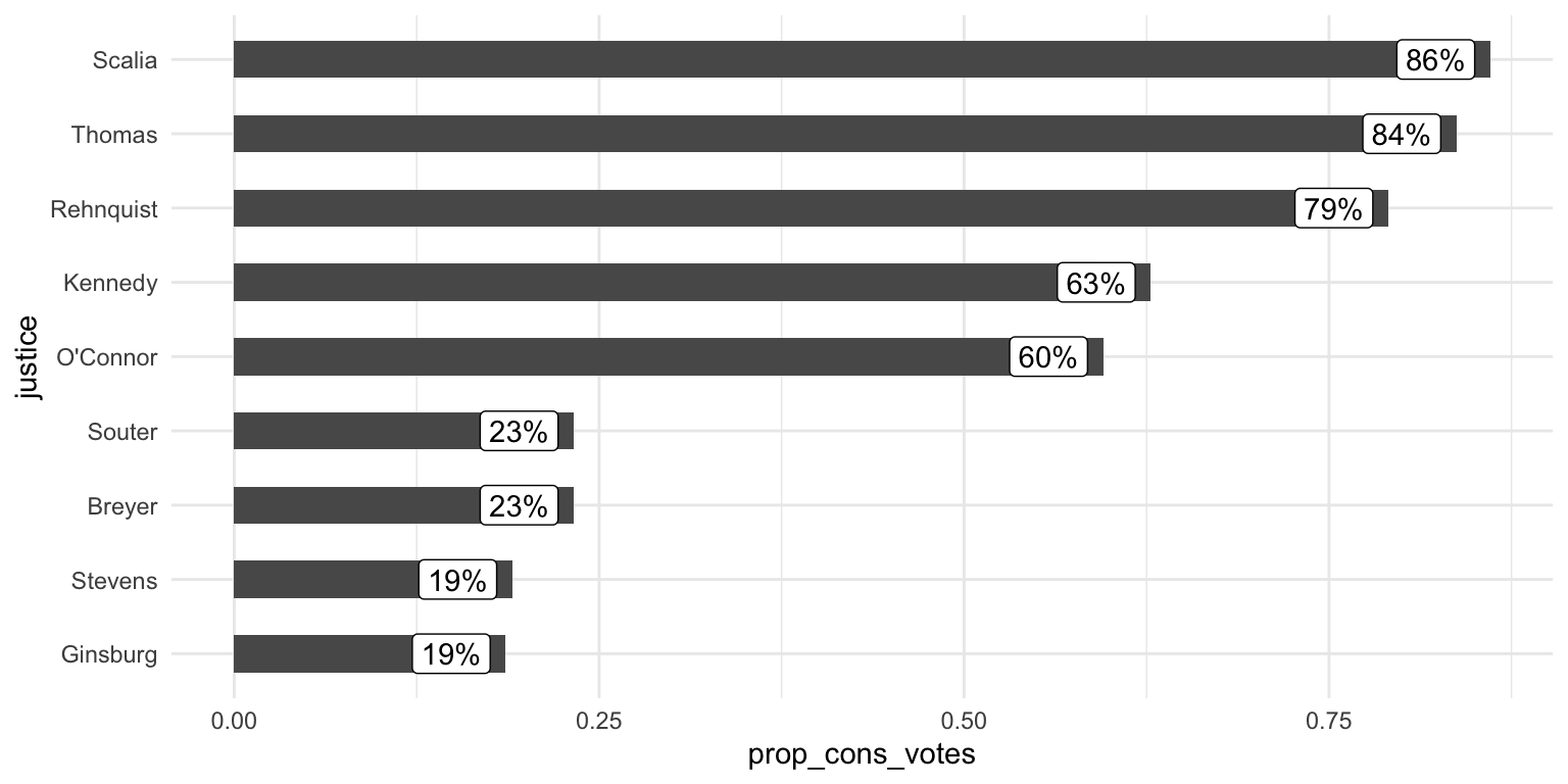
Plot 2
Code
library(ggrepel)

set.seed(1234)
ggplot(sc_summary, aes(x = prop_cons_votes, y = 0)) +
  geom_hline(yintercept = 0) +
  geom_point(size = 3) +
  geom_label_repel(
    aes(label = justice),
    nudge_y = rep_len(c(-1, 1)*0.035, 9),
    segment.color = "grey50",
    direction = "y",
    point.padding = 0.5,
    min.segment.length = 0.0
  ) +
  scale_x_continuous(labels = scales::percent_format(accuracy = 1)) +
  theme_minimal(base_size = 14) +
  theme(
    axis.title.y = element_blank(),
    axis.text.y  = element_blank(),
    axis.ticks.y = element_blank()
  ) +
  labs(
    x = "Proportion of Conserative Votes"
    ) +
  scale_y_continuous(limits = c(-.1, .1))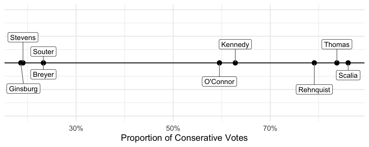
Plot the abilities
Code
ip <- ranef(fit)$justice |>
  as_tibble(rownames = "justice") |>
  rename(ideal_point = `(Intercept)`) |>
  arrange(ideal_point)

set.seed(1234)
ggplot(ip, aes(x = ideal_point, y = 0)) +
  geom_hline(yintercept = 0) +
  geom_point(size = 3) +
  geom_label_repel(
    aes(label = justice),
    nudge_y = rep_len(c(-1, 1)*0.035, 9),
    segment.color = "grey50",
    direction = "y",
    point.padding = 0.5,
    min.segment.length = 0.0
  ) +
  theme_minimal(base_size = 14) +
  theme(
    axis.title.y = element_blank(),
    axis.text.y  = element_blank(),
    axis.ticks.y = element_blank()
  ) +
  labs(
    x = "Ideal Point"
    ) +
  scale_y_continuous(limits = c(-.1, .1))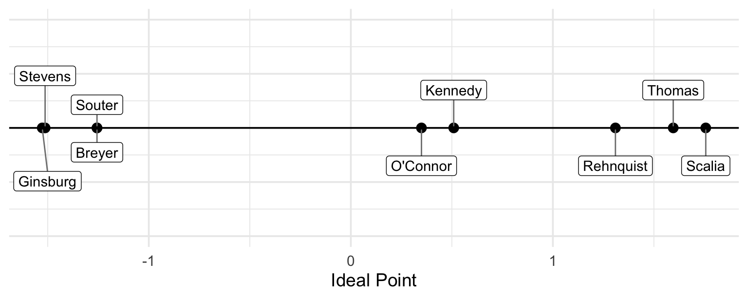
Add cases
Code
library(ggbeeswarm)

cases <- data.frame(case = as.numeric(ranef(fit)$case_id[, "(Intercept)"]))

set.seed(1234)
ggplot(ip, aes(y = ideal_point, x = 0)) +
  geom_vline(xintercept = 0) +
  geom_beeswarm(data = cases, aes( y = case, x = 0), shape = 18, alpha = 0.3, color = "red") +
  geom_beeswarm(size = 2, alpha = 0.5) +
  geom_label_repel(
    aes(label = justice),
    nudge_x = rep_len(c(-1, 1)*0.035, 9),
    segment.color = "grey50",
    direction = "x",
    point.padding = 0.5,
    min.segment.length = 0.0
  ) +
  theme_minimal(base_size = 14) +
  theme(
    axis.title.y = element_blank(),
    axis.text.y  = element_blank(),
    axis.ticks.y = element_blank()
  ) +
  labs(
    x = "Ideal Point"
    ) +
  scale_x_continuous(limits = c(-.1, .1)) +
  coord_flip()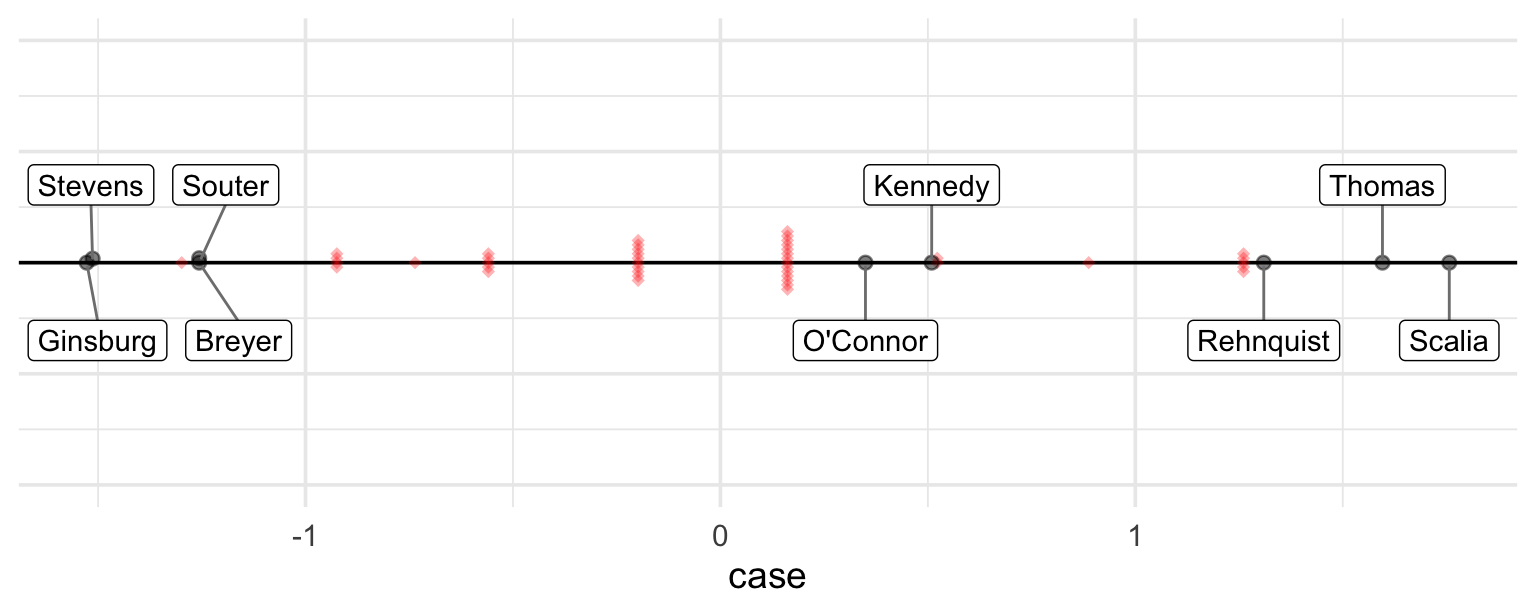
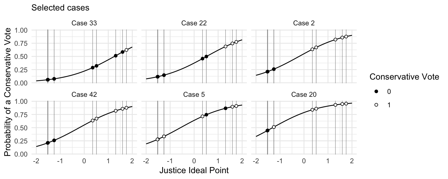
Plot the logit curve
Code
mu <- as.numeric(fixef(fit))

beta <- ranef(fit)$case_id |>
  as_tibble(rownames = "case_id") |>
  rename(beta = `(Intercept)`)

cases_to_keep <- c("Case 20", "Case 5", "Case 2", "Case 42", "Case 22", "Case 33")

pred_lines <- crossing(justice_ideology = seq(-2, 2, length.out = 100),
                      case_id = unique(sc$case_id)) |>
  left_join(beta) |>
  mutate(pr_cons_vote = plogis(mu + justice_ideology + beta)) |>
  mutate(case_id = reorder(case_id, pr_cons_vote)) |>
  filter(case_id %in% cases_to_keep)

pred_points <- sc |>
  left_join(beta) |>
  left_join(ip) |>
  mutate(pr_cons_vote = plogis(mu + ideal_point + beta)) |>
  mutate(case_id = reorder(case_id, pr_cons_vote)) |>
    filter(case_id %in% cases_to_keep)

ggplot(pred_lines, aes(x = justice_ideology, y = pr_cons_vote)) +
  geom_vline(xintercept = ip$ideal_point, color = "grey50", linewidth = 0.2) +
  geom_line() +
  geom_point(data = pred_points, aes(x = ideal_point, y = pr_cons_vote, shape = factor(cons_vote)), fill = "white") +
  facet_wrap(vars(case_id)) +
  scale_shape_manual(values = c(19, 21)) +
  labs(subtitle = "Selected cases",
       shape = "Conservative Vote",
       y = "Probability of a Conservative Vote",
       x = "Justice Ideal Point")