IRT

Opening Comments

Workshop
- When would be a good week for rehearsals and workshops? I’m going to be giving RIBC students extra credit to attend.
Paper

Here are the packages we’re using:

# generally useful packages
library(tidyverse)
library(marginaleffects)
library(modelsummary)

# for fitting hierarchical models
library(lme4)
library(brms)  # see also rstanarm::stan_lmer()
library(rstan)

# for post-processing simulations
library(tidybayes)

# preferred order (most preferred first):
library(conflicted)
conflict_prefer_all("dplyr", quiet = TRUE) 
conflict_prefer_all("tidyr", quiet = TRUE)
conflict_prefer_all("tidybayes", quiet = TRUE) 
conflict_prefer_all("brms", quiet = TRUE)
conflict_prefer_all("rstan", quiet = TRUE)
conflict_prefer_all("patchwork", quiet = TRUE)

Rich State, Poor State, Red State, Blue State

Variables

state_name: U.S. state name joined from state_income by FIPS state_code.
state_median_income State median household income (in thousands of 2024 dollars) from state_income. Example: 92.1 = $92,100.
rs_state_median_income: Rescaled version of state_median_income using arm::rescale() (mean 0, SD 0.5).; i.e.,

income: Numeric scores corresponding to income brackets so that (1) higher numeric values indicate higher household income and (2) the middle is zero.

ANES Category	Income Range (2024 USD)	Recode
1	Under $9,999	−2.5
2	$10,000–$29,999	−1.5
3	$30,000–$59,999	−0.5
4	$60,000–$99,999	0.5
5	$100,000–$249,999	1.5
6	$250,000 or more	2.5

vote_rep: 0/1 indicator of voting for the Republican candidate Donald Trump. Derived from ANES presidential vote V242067 after filtering to major-party voters only.

Results

# load data
anes <- read_csv("data/red-state.csv") |>
  glimpse()

Rows: 3,365
Columns: 5
$ state_name             <chr> "Oklahoma", "Virginia", "Colorado", "Wisconsin", "Wiscons…
$ state_median_income    <dbl> 66.1, 92.1, 97.1, 77.5, 77.5, 92.1, 81.1, 104.8, 99.8, 81…
$ rs_state_median_income <dbl> -0.5953, 0.4122, 0.6060, -0.1536, -0.1536, 0.4122, -0.014…
$ income                 <dbl> 1.5, 1.5, -0.5, -0.5, 1.5, 2.5, -0.5, 2.5, 1.5, 0.5, 1.5,…
$ vote_rep               <dbl> 1, 0, 1, 1, 0, 0, 1, 0, 0, 0, 0, 0, 1, 0, 0, 1, 0, 0, 0, …

# formula
f <- vote_rep ~ rs_state_median_income*income + (1 + income | state_name)

Fit model.

Code

# fit hierarchical model
fit <- brm(
  f,
  data = anes,
  family = bernoulli, 
  chains = 10, 
  cores = 10, 
  iter = 1000
)

Use predictions() to generate

\[ E(\text{Vote R} \mid \text{Individual Income}, \text{State Income}). \]

Code

# state values 
states <- anes %>%
  dplyr::select(state_name, state_median_income, rs_state_median_income) %>%
  distinct() %>%
  glimpse()

Rows: 51
Columns: 3
$ state_name             <chr> "Oklahoma", "Virginia", "Colorado", "Wisconsin", "Nevada"…
$ state_median_income    <dbl> 66.1, 92.1, 97.1, 77.5, 81.1, 104.8, 99.8, 85.8, 80.0, 81…
$ rs_state_median_income <dbl> -0.59534, 0.41222, 0.60598, -0.15357, -0.01406, 0.90437, …

Code

# expected values
grid <- crossing(state_name = unique(anes$state_name)) |>
  left_join(states) |>
  mutate(income = NA) |>
  glimpse()

Rows: 51
Columns: 4
$ state_name             <chr> "Alabama", "Alaska", "Arizona", "Arkansas", "California",…
$ state_median_income    <dbl> 66.7, 95.7, 81.5, 62.1, 100.1, 97.1, 96.0, 87.5, 109.7, 7…
$ rs_state_median_income <dbl> -0.57209, 0.55173, 0.00144, -0.75035, 0.72224, 0.60598, 0…
$ income                 <lgl> NA, NA, NA, NA, NA, NA, NA, NA, NA, NA, NA, NA, NA, NA, N…

Code

p <- predictions(fit, 
                 variables = list(income = unique),
                 newdata = grid) |>
  left_join(states) |>
  mutate(state_name = reorder(state_name, rs_state_median_income))

Plotting the estimates

What’s going on here?

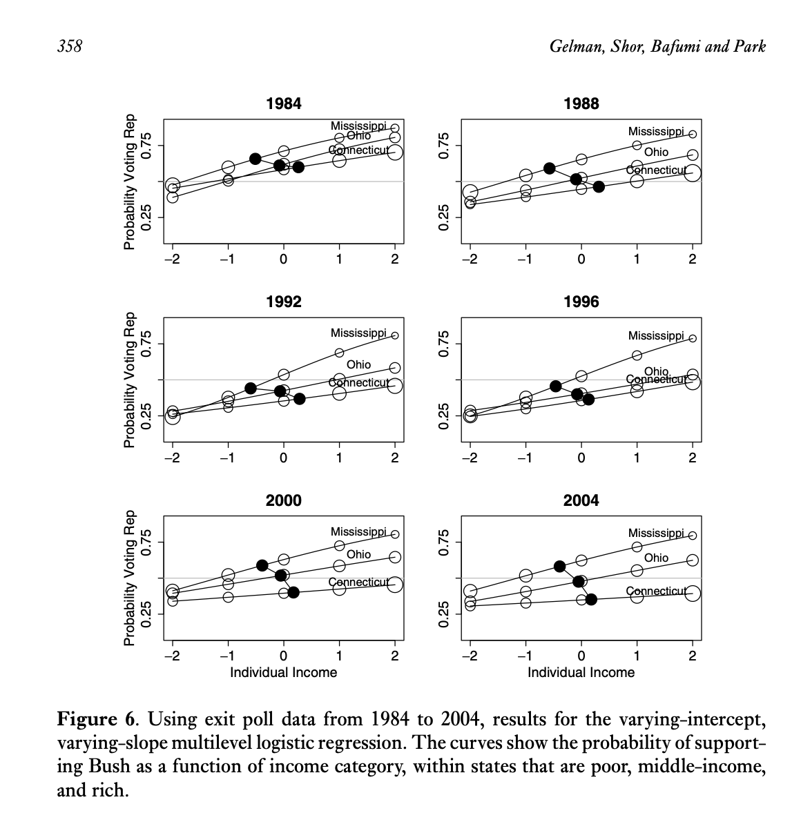
Code

ggplot(p, aes(x = income, y = estimate, group = state_name, color = state_median_income)) + 
  geom_line() + 
  labs(x = "Income Category", 
       y = "Probability of Voting for Trump", 
       title = "Probability of Voting for Trump", 
       subtitle = "States Plotted Together; Color Shows Median Income", 
       color = "State Income") + 
  theme(legend.position = "bottom")

Tappin (2023)

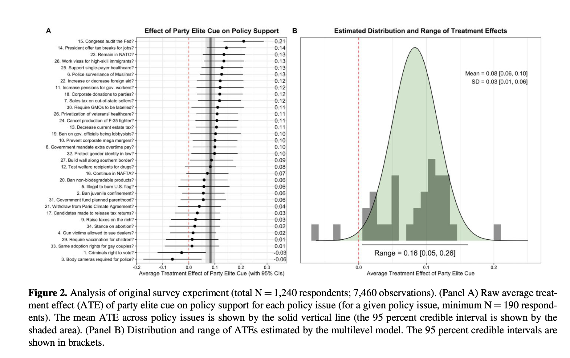
Data

outcome_recode_01 is the outcome variable
cue is the treatment indicator
item indexes the policy
pid indexes respondents.

Code

# load Tappin's (2023) data
# - from https://osf.io/t2bpj/
df <- read_rds("data/open_data.rds") 

# following Tappin, do a little wrangling
# - from analysis__original_exp.R at https://osf.io/t2bpj/
df_for_model <-
  df %>%
  filter(continue_check == 2, 
         item %in% c(1:34)) %>% 
  filter(pol_party != 4) %>% 
  dplyr::select(pid, 
         outcome_recode_01, 
         cue, 
         item, 
         item_label, 
         word_captcha, 
         policy_group, 
         order_variable) %>%
  filter(!is.na(outcome_recode_01)) |>
  glimpse()

Rows: 7,460
Columns: 8
$ pid               <int> 5, 5, 5, 5, 5, 7, 7, 7, 7, 7, 7, 7, 8, 8, 8, 8, 8, 8, 8, 8, 10…
$ outcome_recode_01 <dbl> 0.833, 0.667, 0.000, 0.667, 0.167, 0.667, 0.500, 1.000, 0.500,…
$ cue               <int> 0, 1, 0, 1, 0, 1, 0, 0, 0, 0, 1, 0, 1, 0, 0, 1, 1, 1, 1, 0, 0,…
$ item              <dbl> 1, 4, 6, 9, 18, 1, 4, 5, 13, 14, 30, 34, 4, 5, 8, 17, 20, 25, …
$ item_label        <chr> "1. Criminals right to vote?", "4. Gun victims allowed to sue …
$ word_captcha      <chr> "hello", "hello", "hello", "hello", "hello", "hello", "hello",…
$ policy_group      <chr> "Crime", "Domestic policy", "Domestic policy", "Economy", "Ele…
$ order_variable    <dbl> 4, 1, 6, 8, 5, 2, 4, 6, 3, 7, 5, 1, 4, 6, 8, 2, 7, 3, 1, 5, 2,…

Fit models

Fit linear model; do {marginaleffects}.

Code

ls_fit <- lm(outcome_recode_01 ~ item_label*cue, data = df_for_model)

c <- comparisons(ls_fit, 
                 variables = list(cue = c(0, 1)), 
                 newdata = datagrid(item_label = unique)) |>
  mutate(item_label = reorder(item_label, estimate)) |>
  mutate(model = "No Pooling; Least Squares")

Fit hierarchical model.

Code

brm_fit <- brm(outcome_recode_01 ~ 1 + cue + (1 + cue | item_label), 
               data = df_for_model, 
               chains = 10, 
               cores = 10, 
               iter = 1000)

Do {marginaleffects}; combine with above.

Code

c2 <- comparisons(brm_fit, 
                 variables = list(cue = c(0, 1)), 
                 newdata = datagrid(item_label = unique)) |>
  mutate(item_label = reorder(item_label, estimate)) |>
  mutate(model = "Hierarchical") |>
  bind_rows(c)

Plot estimates

Code

ggplot(c2, aes(x = estimate, 
               y = item_label, 
               xmin = conf.low, 
               xmax = conf.high, 
               color = model)) + 
  geom_pointrange(position = ggstance::position_dodgev(height = 0.6), 
                  size = 0.2)

IRT

This week, I introduce the idea of a IRT model.

This is just one specific type of hierarchical model.

The `answers` data

The answers dataset has answers from hypothetical students to real questions from a recent exam.

question_id_num indexes the 55 questions on the exam.
student_id_num indexes the 100 students who took the exam.
correct_answer indicates (0/1) where the student answered the question correctly.

answers <- read_csv("https://pos5747.github.io/data/example-answers.csv") |>
  glimpse()

Rows: 5,500
Columns: 3
$ student_id_num  <dbl> 1, 1, 1, 1, 1, 1, 1, 1, 1, 1, 1, 1, 1, 1, 1, 1, 1, 1, 1, 1, 1, 1…
$ question_id_num <dbl> 1, 2, 3, 4, 5, 6, 7, 8, 9, 10, 11, 12, 13, 14, 15, 16, 17, 18, 1…
$ correct_answer  <dbl> 1, 1, 1, 1, 1, 1, 1, 1, 1, 1, 1, 1, 1, 1, 0, 1, 1, 1, 1, 1, 1, 1…

Grades on the exam

grades <- answers %>% 
  group_by(student_id_num) %>%
  summarize(proportion_correct = mean(correct_answer)) %>%
  mutate(
    letter_grade = cut(
      proportion_correct,
      breaks = c(-Inf, 0.60, 0.63, 0.67, 0.70, 0.73, 0.77, 0.80, 0.83, 0.87, 0.90, 0.93, Inf),
      labels = c("F",  "D-", "D",  "D+", "C-", "C",  "C+", "B-", "B",  "B+", "A-", "A"),
      ordered_result = TRUE
    )
  )

grades |> filter(student_id_num <= 10)

# A tibble: 10 × 3
   student_id_num proportion_correct letter_grade
            <dbl>              <dbl> <ord>       
 1              1              0.909 A-          
 2              2              0.527 F           
 3              3              0.764 C           
 4              4              0.727 C-          
 5              5              0.964 A           
 6              6              0.818 B-          
 7              7              0.818 B-          
 8              8              0.782 C+          
 9              9              0.564 F           
10             10              0.8   C+

Rasch / 1-PL model

Indices

Answers: $n = 1, \dots, N$. ($N = 55 \times 100 = 5{,}500$ in our data.)
Students: $j = 1, \dots, J$. ($J = 100$ in our data.)
Questions: $k = 1, \dots, K$. ($K = 55$ in our data.)

Outcome: $y_{n} \in \{0, 1\}$ indicates whether the $n$th answer is correct.

\[ y_n \sim \mathrm{Bernoulli}(\pi_n) \\ \pi_n = \text{logit}^{-1} \left( \mu + \alpha_{j[n]} - \beta_{k[n]} \right). \]

Parameters

$\pi_n$: the probability that answer $n$ is correct
$\alpha_{j[n]}$: the ability of student $j$ [who is giving the $n$th answer].
- Higher $\alpha_j$ ⇒ more likely to answer correctly; more knowledgeable student.
$\beta_{k[n]}$: the difficulty of question $k$ [which is associated with the $n$th answer].
- Higher $\beta_k$ ⇒ less likely to answer correctly; harder item.
$\mu$: average difficulty across questions

Hierarchical Model

\[ \alpha_j \sim N(0,\sigma_\alpha^2)\\ \beta_k \sim N(0,\sigma_\beta^2) \]

Priors

\[ \sigma_\alpha \sim \mathrm{half\text{-}Cauchy}(0,1)\\ \sigma_\beta \sim \mathrm{half\text{-}Cauchy}(0,1) \]

\[ \mu \sim \mathrm{Cauchy}(0,1). \]

A change from 0 to 1 on the logit scale increase the chance of success from 50% to 73%. A change from 1 to 2 increases the chance of success from 73% to 88%.

plogis(0); plogis(1); plogis(2)

[1] 0.5

[1] 0.731

[1] 0.881

$\sigma_\alpha = 1$ means that the “give or take” on the abilities is about 1.
Suppose an average student has a 73% change of answering a given question correctly. If $\sigma_\alpha = 1$, then “most” (68%) students have between a 50% and 88% chance of answering correctly. This seems “about right” to me, so I expect $\sigma_\alpha$ to be about 1 (i.e., not 0.1 or 10).
The median of a half-Cauchy is the scale, so I set the scale to the $\sigma_\alpha$ that seems “about right.”
This is a somewhat aggressive prior that polls the variances toward zero—I want to treat bias the model toward treating students and questions as “similar”. Setting the scale to 2.5 or 5 is more conservative.

Stan model

data {
  int<lower=1> N;  // number of answers
  int<lower=1> J;  // number of students
  int<lower=1> K;  // number of questions
  int<lower=1, upper=J> jj[N];  // student index for answer n
  int<lower=1, upper=K> kk[N];  // question index for answer n
  int<lower=0, upper=1> y[N];  // answer n is correct (0/1)
}

parameters {
  real mu;  // mean difficulty
  vector[J] alpha;  // abilities; one per student
  vector[K] beta;  // difficulties; one per question
  real<lower=0> sigma_beta;  // SD of difficulties
  real<lower=0> sigma_alpha;  // SD of abilities
}

model {
  sigma_beta ~ cauchy(0, 1);  // prior for SD of difficulties
  sigma_alpha ~ cauchy(0, 1);  // prior for SD of abilities
  mu ~ cauchy(0, 1);  // prior for mean difficulty
  alpha ~ normal(0, sigma_alpha);  // abilities
  beta ~ normal(0, sigma_beta);  // difficulties
  for (n in 1:N) {
    y[n] ~ bernoulli_logit(mu + alpha[jj[n]] - beta[kk[n]]);  // likelihood
  }
}

Set up data for Stan

# make data for stan
data_list <- list(
  # upper bounds of indices
  N = nrow(answers),                 # - n in {1,...,N} indexes answers
  J = max(answers$student_id_num),   # - j in {1,...,J} indexes students
  K = max(answers$question_id_num),  # - k in {1,...,K} indexes questions
  # indices for each respondent
  jj = answers$student_id_num,   # jj is a vector of student indices for each answer
  kk = answers$question_id_num,  # kk is a vector of question indices for each answer
  # observed answers
  y = answers$correct_answer
)

jj and kk are subtle!

Because all students answer all questions, we have $N = 100 \times 55 = 5,500$ answers.
jj and kk are both length-$N$ vectors.
jj[n] tells us the student who gave the $n$th answer.
kk[n] tells us the question that goes with the $n$th answer.

What do these data look like?

n <- 1:5500
look_at_n <- c(1, 10, 55, 100, 1000, 2000, 5500) # answers to look at
cbind("n" = n, "jj" = data_list$jj, "kk" = data_list$kk, "y" = data_list$y)[look_at_n, ]

        n  jj kk y
[1,]    1   1  1 1
[2,]   10   1 10 1
[3,]   55   1 55 1
[4,]  100   2 45 1
[5,] 1000  19 10 0
[6,] 2000  37 20 1
[7,] 5500 100 55 0

A trick

I like to create a character string that has the Stan model, so that it’s right in my R script. (Or you can create a file.)

stan_code <- "
data {
  int<lower=1> N;  // number of answers
  int<lower=1> J;  // number of students
  int<lower=1> K;  // number of questions
  int<lower=1, upper=J> jj[N];  // student index for answer n
  int<lower=1, upper=K> kk[N];  // question index for answer n
  int<lower=0, upper=1> y[N];  // answer n is correct (0/1)
}

parameters {
  real mu;  // mean difficulty
  vector[J] alpha;  // abilities; one per student
  vector[K] beta;  // difficulties; one per question
  real<lower=0> sigma_beta;  // SD of difficulties
  real<lower=0> sigma_alpha;  // SD of abilities
}

model {
  sigma_beta ~ cauchy(0, 1);  // prior for SD of difficulties
  sigma_alpha ~ cauchy(0, 1);  // prior for SD of abilities
  mu ~ cauchy(0, 1);  // prior for mean difficulty
  alpha ~ normal(0, sigma_alpha);  // abilities
  beta ~ normal(0, sigma_beta);  // difficulties
  for (n in 1:N) {
    y[n] ~ bernoulli_logit(mu + alpha[jj[n]] - beta[kk[n]]);  // likelihood
  }
}
"

Fit Stan model using {rstan}

start_time <- Sys.time()

fit <- stan(model_code = stan_code, 
            data = data_list,
            iter = 1000, 
            warmup = 500,
            chains = 10, 
            cores = 10)
            
end_time <- Sys.time()

Print the `fit`

Was iter large enough?

print(fit)

Inference for Stan model: anon_model.
10 chains, each with iter=1000; warmup=500; thin=1; 
post-warmup draws per chain=500, total post-warmup draws=5000.

                mean se_mean   sd     2.5%      25%      50%      75%    97.5% n_eff Rhat
mu              1.34    0.01 0.14     1.06     1.25     1.35     1.44     1.63   557 1.03
alpha[1]        0.97    0.01 0.42     0.18     0.68     0.96     1.25     1.82  4378 1.00
alpha[2]       -1.14    0.01 0.29    -1.69    -1.33    -1.14    -0.95    -0.57  2877 1.00
alpha[3]       -0.04    0.01 0.33    -0.68    -0.27    -0.05     0.17     0.64  3551 1.00
alpha[4]       -0.24    0.01 0.32    -0.86    -0.45    -0.24    -0.02     0.41  3690 1.00
alpha[5]        1.58    0.01 0.50     0.67     1.24     1.56     1.90     2.64  5901 1.00
alpha[6]        0.28    0.01 0.35    -0.36     0.04     0.27     0.52     0.98  4031 1.00
alpha[7]        0.29    0.01 0.35    -0.38     0.05     0.28     0.52     0.99  4187 1.00
alpha[8]        0.06    0.01 0.34    -0.57    -0.17     0.06     0.29     0.73  3995 1.00
alpha[9]       -0.98    0.01 0.30    -1.56    -1.19    -0.99    -0.79    -0.39  2797 1.00
alpha[10]       0.17    0.01 0.34    -0.49    -0.06     0.17     0.39     0.85  3771 1.00
alpha[11]       0.53    0.01 0.38    -0.17     0.26     0.52     0.78     1.31  3818 1.00
alpha[12]      -0.75    0.01 0.30    -1.32    -0.94    -0.75    -0.55    -0.18  3446 1.00
alpha[13]      -0.14    0.01 0.33    -0.77    -0.36    -0.15     0.07     0.51  3635 1.00
alpha[14]       1.57    0.01 0.50     0.66     1.22     1.55     1.90     2.62  5693 1.00
alpha[15]       0.17    0.01 0.34    -0.46    -0.07     0.17     0.39     0.86  3965 1.00
alpha[16]      -0.42    0.01 0.31    -1.01    -0.62    -0.42    -0.21     0.20  3368 1.00
alpha[17]      -0.74    0.01 0.30    -1.30    -0.95    -0.75    -0.54    -0.15  3454 1.00
alpha[18]       1.58    0.01 0.50     0.66     1.23     1.56     1.91     2.62  5288 1.00
alpha[19]       1.16    0.01 0.45     0.35     0.85     1.14     1.45     2.08  5042 1.00
alpha[20]       0.53    0.01 0.37    -0.19     0.27     0.52     0.78     1.27  4335 1.00
alpha[21]      -0.14    0.01 0.33    -0.76    -0.36    -0.14     0.08     0.53  3753 1.00
alpha[22]      -2.06    0.01 0.31    -2.67    -2.26    -2.06    -1.85    -1.46  2549 1.00
alpha[23]      -0.67    0.01 0.30    -1.24    -0.87    -0.67    -0.47    -0.07  3417 1.00
alpha[24]      -0.75    0.01 0.30    -1.33    -0.95    -0.75    -0.55    -0.17  3112 1.00
alpha[25]       0.17    0.01 0.35    -0.49    -0.07     0.16     0.40     0.88  4058 1.00
alpha[26]       2.14    0.01 0.60     1.07     1.72     2.10     2.51     3.43  4606 1.00
alpha[27]      -0.58    0.01 0.30    -1.18    -0.78    -0.59    -0.38     0.01  3461 1.00
alpha[28]       0.97    0.01 0.42     0.21     0.68     0.95     1.24     1.84  4386 1.00
alpha[29]       1.36    0.01 0.46     0.52     1.04     1.35     1.66     2.31  4991 1.00
alpha[30]       0.97    0.01 0.40     0.24     0.69     0.95     1.23     1.78  4799 1.00
alpha[31]       0.82    0.01 0.41     0.06     0.53     0.80     1.09     1.65  4600 1.00
alpha[32]       1.59    0.01 0.52     0.66     1.23     1.57     1.91     2.70  5250 1.00
alpha[33]       0.98    0.01 0.42     0.20     0.68     0.97     1.25     1.83  5633 1.00
alpha[34]       0.82    0.01 0.40     0.06     0.54     0.80     1.07     1.62  4194 1.00
alpha[35]       1.36    0.01 0.46     0.51     1.03     1.34     1.65     2.29  4785 1.00
alpha[36]      -0.41    0.01 0.31    -1.03    -0.63    -0.41    -0.20     0.21  2993 1.00
alpha[37]      -0.50    0.01 0.31    -1.10    -0.71    -0.51    -0.29     0.13  3877 1.00
alpha[38]      -0.90    0.01 0.29    -1.47    -1.10    -0.90    -0.71    -0.34  2953 1.00
alpha[39]       0.53    0.01 0.37    -0.17     0.28     0.52     0.78     1.29  3889 1.00
alpha[40]      -0.50    0.01 0.32    -1.10    -0.72    -0.50    -0.29     0.11  3330 1.00
alpha[41]      -1.36    0.01 0.30    -1.94    -1.56    -1.36    -1.16    -0.78  3004 1.00
alpha[42]       0.97    0.01 0.42     0.18     0.69     0.96     1.24     1.82  3878 1.00
alpha[43]      -0.41    0.01 0.31    -0.98    -0.62    -0.41    -0.20     0.21  2351 1.00
alpha[44]       0.97    0.01 0.43     0.18     0.68     0.96     1.24     1.86  4512 1.00
alpha[45]       0.98    0.01 0.42     0.20     0.69     0.96     1.25     1.83  4889 1.00
alpha[46]       0.41    0.01 0.36    -0.27     0.17     0.39     0.65     1.15  3600 1.00
alpha[47]       0.41    0.01 0.36    -0.26     0.17     0.39     0.64     1.13  3198 1.00
alpha[48]      -0.04    0.01 0.34    -0.68    -0.26    -0.04     0.18     0.65  3599 1.00
alpha[49]      -1.05    0.01 0.29    -1.63    -1.25    -1.06    -0.86    -0.47  3242 1.00
alpha[50]      -1.21    0.01 0.29    -1.79    -1.41    -1.21    -1.01    -0.64  2767 1.00
alpha[51]      -0.23    0.01 0.32    -0.84    -0.46    -0.23    -0.02     0.40  3024 1.00
alpha[52]      -0.05    0.01 0.33    -0.66    -0.27    -0.06     0.17     0.60  3787 1.00
alpha[53]      -1.13    0.01 0.29    -1.69    -1.34    -1.14    -0.94    -0.55  3170 1.00
alpha[54]      -0.67    0.01 0.32    -1.27    -0.89    -0.68    -0.46    -0.04  3103 1.00
alpha[55]       0.41    0.01 0.37    -0.27     0.16     0.40     0.65     1.17  4837 1.00
alpha[56]       0.28    0.01 0.36    -0.38     0.04     0.27     0.52     1.02  4000 1.00
alpha[57]       0.52    0.01 0.37    -0.19     0.27     0.51     0.77     1.27  3784 1.00
alpha[58]      -1.89    0.01 0.30    -2.51    -2.09    -1.90    -1.69    -1.31  2827 1.00
alpha[59]       0.81    0.01 0.40     0.05     0.53     0.80     1.07     1.65  5544 1.00
alpha[60]      -0.14    0.01 0.33    -0.77    -0.36    -0.15     0.08     0.50  4026 1.00
alpha[61]      -0.58    0.01 0.30    -1.18    -0.79    -0.58    -0.38     0.03  3077 1.00
alpha[62]      -0.42    0.01 0.31    -1.02    -0.63    -0.42    -0.22     0.19  2684 1.00
alpha[63]      -0.23    0.01 0.32    -0.85    -0.44    -0.23    -0.02     0.40  2679 1.00
alpha[64]       0.17    0.01 0.34    -0.48    -0.06     0.17     0.40     0.87  4265 1.00
alpha[65]       1.58    0.01 0.50     0.66     1.24     1.56     1.89     2.63  5581 1.00
alpha[66]      -0.23    0.01 0.33    -0.85    -0.46    -0.24    -0.01     0.41  4193 1.00
alpha[67]      -2.41    0.01 0.32    -3.05    -2.62    -2.40    -2.19    -1.80  3350 1.00
alpha[68]      -1.06    0.01 0.29    -1.63    -1.26    -1.06    -0.86    -0.48  2919 1.00
alpha[69]      -1.13    0.01 0.29    -1.69    -1.33    -1.14    -0.94    -0.55  3101 1.00
alpha[70]      -1.13    0.01 0.30    -1.70    -1.33    -1.13    -0.94    -0.53  2662 1.00
alpha[71]       0.40    0.01 0.36    -0.27     0.15     0.39     0.65     1.11  3684 1.00
alpha[72]      -0.32    0.01 0.32    -0.94    -0.53    -0.32    -0.11     0.32  2868 1.00
alpha[73]       0.98    0.01 0.42     0.17     0.69     0.96     1.25     1.83  5748 1.00
alpha[74]      -0.41    0.01 0.32    -1.03    -0.63    -0.42    -0.20     0.23  3401 1.00
alpha[75]      -0.24    0.01 0.32    -0.86    -0.45    -0.24    -0.03     0.41  2986 1.00
alpha[76]      -0.24    0.01 0.32    -0.84    -0.45    -0.24    -0.02     0.38  3580 1.00
alpha[77]       1.35    0.01 0.48     0.47     1.01     1.33     1.66     2.34  5266 1.00
alpha[78]      -1.29    0.01 0.30    -1.85    -1.50    -1.29    -1.09    -0.72  2442 1.00
alpha[79]       0.17    0.01 0.34    -0.47    -0.06     0.16     0.40     0.88  3514 1.00
alpha[80]      -0.23    0.01 0.32    -0.83    -0.46    -0.24    -0.01     0.40  3355 1.00
alpha[81]      -0.24    0.01 0.32    -0.86    -0.45    -0.24    -0.02     0.42  3471 1.00
alpha[82]       0.67    0.01 0.39    -0.06     0.40     0.66     0.93     1.45  5057 1.00
alpha[83]      -0.59    0.01 0.31    -1.20    -0.79    -0.59    -0.38     0.02  3290 1.00
alpha[84]      -0.91    0.01 0.30    -1.49    -1.10    -0.91    -0.71    -0.32  2866 1.00
alpha[85]      -0.83    0.01 0.30    -1.40    -1.03    -0.83    -0.63    -0.23  3169 1.00
alpha[86]      -0.49    0.01 0.32    -1.10    -0.71    -0.50    -0.28     0.13  3314 1.00
alpha[87]       1.35    0.01 0.47     0.49     1.02     1.33     1.65     2.32  4899 1.00
alpha[88]       0.28    0.01 0.35    -0.39     0.04     0.27     0.52     1.00  4031 1.00
alpha[89]       0.07    0.01 0.34    -0.58    -0.17     0.06     0.29     0.74  3448 1.00
alpha[90]       0.40    0.01 0.36    -0.29     0.16     0.40     0.63     1.15  4135 1.00
alpha[91]       1.85    0.01 0.55     0.87     1.46     1.82     2.19     3.01  4415 1.00
alpha[92]      -0.75    0.01 0.31    -1.34    -0.96    -0.75    -0.54    -0.14  3242 1.00
alpha[93]       0.53    0.01 0.38    -0.16     0.27     0.51     0.78     1.32  3817 1.00
alpha[94]      -0.04    0.01 0.33    -0.68    -0.26    -0.04     0.18     0.61  3685 1.00
alpha[95]      -0.22    0.01 0.32    -0.81    -0.44    -0.23    -0.01     0.43  3278 1.00
alpha[96]      -1.66    0.01 0.29    -2.25    -1.85    -1.67    -1.47    -1.10  3193 1.00
alpha[97]      -0.67    0.01 0.30    -1.24    -0.87    -0.66    -0.46    -0.08  3111 1.00
alpha[98]      -0.14    0.01 0.32    -0.75    -0.35    -0.14     0.08     0.50  3964 1.00
alpha[99]       0.07    0.01 0.33    -0.56    -0.16     0.06     0.28     0.74  3667 1.00
alpha[100]     -0.23    0.01 0.32    -0.83    -0.45    -0.24    -0.03     0.41  3328 1.00
beta[1]        -0.66    0.00 0.28    -1.23    -0.85    -0.66    -0.47    -0.12  4318 1.00
beta[2]        -0.91    0.00 0.30    -1.52    -1.11    -0.90    -0.69    -0.35  3656 1.00
beta[3]        -0.14    0.00 0.26    -0.66    -0.31    -0.14     0.03     0.37  3409 1.00
beta[4]        -0.26    0.00 0.26    -0.78    -0.43    -0.25    -0.08     0.23  3450 1.00
beta[5]        -0.14    0.00 0.26    -0.64    -0.31    -0.14     0.04     0.35  3380 1.00
beta[6]         0.14    0.00 0.24    -0.34    -0.02     0.15     0.31     0.61  3039 1.00
beta[7]         0.49    0.00 0.24     0.01     0.33     0.49     0.65     0.96  3088 1.00
beta[8]        -0.82    0.01 0.31    -1.46    -1.01    -0.81    -0.60    -0.24  3788 1.00
beta[9]        -0.73    0.00 0.29    -1.31    -0.92    -0.73    -0.53    -0.19  3537 1.00
beta[10]        0.45    0.00 0.24    -0.03     0.28     0.45     0.61     0.90  2910 1.00
beta[11]       -0.32    0.00 0.27    -0.86    -0.49    -0.31    -0.14     0.19  2864 1.00
beta[12]        0.20    0.00 0.24    -0.29     0.04     0.20     0.36     0.69  2486 1.00
beta[13]        0.99    0.00 0.23     0.53     0.84     1.00     1.15     1.46  2907 1.00
beta[14]       -0.20    0.00 0.26    -0.73    -0.37    -0.19    -0.01     0.30  3127 1.00
beta[15]        0.45    0.00 0.24     0.00     0.29     0.44     0.61     0.91  2575 1.00
beta[16]       -0.52    0.00 0.28    -1.07    -0.70    -0.51    -0.32     0.01  3889 1.00
beta[17]       -0.81    0.01 0.30    -1.43    -1.02    -0.81    -0.60    -0.25  3523 1.00
beta[18]       -0.26    0.00 0.26    -0.78    -0.43    -0.25    -0.08     0.22  3187 1.00
beta[19]       -0.66    0.00 0.29    -1.24    -0.85    -0.66    -0.47    -0.13  3753 1.00
beta[20]        0.45    0.00 0.24    -0.03     0.29     0.45     0.61     0.91  2405 1.00
beta[21]       -0.59    0.00 0.28    -1.15    -0.78    -0.59    -0.40    -0.06  3726 1.00
beta[22]        0.09    0.00 0.25    -0.42    -0.09     0.10     0.26     0.58  3018 1.00
beta[23]       -0.60    0.00 0.28    -1.18    -0.78    -0.59    -0.40    -0.06  3762 1.00
beta[24]        0.30    0.00 0.25    -0.19     0.13     0.30     0.46     0.77  2522 1.00
beta[25]       -0.08    0.00 0.26    -0.59    -0.25    -0.07     0.10     0.40  3022 1.00
beta[26]        0.35    0.00 0.25    -0.14     0.19     0.34     0.51     0.82  2654 1.00
beta[27]        1.58    0.00 0.23     1.13     1.42     1.58     1.73     2.03  2653 1.00
beta[28]        1.53    0.00 0.23     1.08     1.37     1.53     1.69     1.99  2978 1.00
beta[29]        0.24    0.00 0.24    -0.23     0.08     0.24     0.40     0.72  3110 1.00
beta[30]       -1.07    0.00 0.31    -1.71    -1.28    -1.06    -0.86    -0.48  4270 1.00
beta[31]        0.09    0.00 0.25    -0.39    -0.07     0.09     0.26     0.57  3315 1.00
beta[32]       -0.90    0.00 0.30    -1.49    -1.10    -0.89    -0.69    -0.32  3971 1.00
beta[33]       -1.17    0.01 0.32    -1.83    -1.38    -1.15    -0.95    -0.56  3781 1.00
beta[34]       -0.90    0.00 0.30    -1.51    -1.10    -0.89    -0.69    -0.32  4263 1.00
beta[35]        0.73    0.00 0.23     0.26     0.58     0.73     0.88     1.18  2707 1.00
beta[36]        0.20    0.00 0.25    -0.30     0.03     0.20     0.37     0.67  2655 1.00
beta[37]       -0.45    0.00 0.27    -0.99    -0.63    -0.44    -0.26     0.07  3636 1.00
beta[38]        0.14    0.00 0.24    -0.33    -0.03     0.14     0.30     0.62  2810 1.00
beta[39]        0.45    0.00 0.24    -0.02     0.29     0.45     0.61     0.93  2398 1.00
beta[40]       -0.89    0.01 0.30    -1.50    -1.09    -0.89    -0.69    -0.34  3335 1.00
beta[41]       -0.38    0.00 0.27    -0.92    -0.56    -0.38    -0.20     0.13  3993 1.00
beta[42]        0.49    0.00 0.24     0.03     0.34     0.49     0.65     0.95  2694 1.00
beta[43]        0.91    0.00 0.23     0.46     0.76     0.91     1.07     1.36  2777 1.00
beta[44]        0.59    0.00 0.24     0.13     0.43     0.59     0.75     1.06  2364 1.01
beta[45]       -0.90    0.00 0.30    -1.49    -1.10    -0.90    -0.69    -0.32  4379 1.00
beta[46]        0.87    0.00 0.23     0.41     0.71     0.86     1.02     1.32  2685 1.00
beta[47]       -0.20    0.00 0.26    -0.72    -0.37    -0.20    -0.02     0.30  3367 1.00
beta[48]        0.09    0.00 0.25    -0.41    -0.08     0.09     0.25     0.57  2740 1.00
beta[49]        1.00    0.00 0.23     0.53     0.84     1.00     1.16     1.45  2553 1.00
beta[50]       -0.26    0.00 0.27    -0.80    -0.44    -0.26    -0.08     0.26  3346 1.00
beta[51]        0.14    0.00 0.24    -0.33    -0.02     0.14     0.31     0.62  2982 1.00
beta[52]        0.78    0.00 0.24     0.31     0.62     0.77     0.94     1.25  2851 1.00
beta[53]        0.68    0.00 0.23     0.22     0.52     0.68     0.84     1.14  2841 1.00
beta[54]       -0.03    0.00 0.26    -0.54    -0.20    -0.02     0.15     0.47  3124 1.00
beta[55]       -0.08    0.00 0.25    -0.58    -0.25    -0.08     0.09     0.41  3272 1.00
sigma_beta      0.71    0.00 0.08     0.57     0.65     0.70     0.76     0.88  4501 1.00
sigma_alpha     0.98    0.00 0.08     0.82     0.91     0.97     1.03     1.15  3229 1.00
lp__        -2656.07    0.20 9.06 -2674.38 -2661.98 -2655.85 -2649.82 -2638.98  2094 1.00

Samples were drawn using NUTS(diag_e) at Wed Nov 12 08:14:38 2025.
For each parameter, n_eff is a crude measure of effective sample size,
and Rhat is the potential scale reduction factor on split chains (at 
convergence, Rhat=1).

Using `spread_draws()` from {tidybayes}

fit %>%
  spread_draws(alpha[student_id_num])

# A tibble: 500,000 × 5
# Groups:   student_id_num [100]
   student_id_num alpha .chain .iteration .draw
            <int> <dbl>  <int>      <int> <int>
 1              1 1.63       1          1     1
 2              1 0.241      1          2     2
 3              1 1.10       1          3     3
 4              1 0.948      1          4     4
 5              1 1.18       1          5     5
 6              1 0.941      1          6     6
 7              1 1.15       1          7     7
 8              1 0.869      1          8     8
 9              1 0.735      1          9     9
10              1 0.908      1         10    10
# ℹ 499,990 more rows

Adding `mean_qi()` from {tidybayes}

fit %>%
  spread_draws(alpha[student_id_num]) %>%
  median_qi()  # works like group_by() |> summarize()

# A tibble: 100 × 7
   student_id_num   alpha .lower .upper .width .point .interval
            <int>   <dbl>  <dbl>  <dbl>  <dbl> <chr>  <chr>    
 1              1  0.959   0.180  1.82    0.95 median qi       
 2              2 -1.14   -1.69  -0.574   0.95 median qi       
 3              3 -0.0507 -0.680  0.643   0.95 median qi       
 4              4 -0.242  -0.858  0.407   0.95 median qi       
 5              5  1.56    0.674  2.64    0.95 median qi       
 6              6  0.266  -0.363  0.980   0.95 median qi       
 7              7  0.278  -0.383  0.994   0.95 median qi       
 8              8  0.0573 -0.573  0.734   0.95 median qi       
 9              9 -0.988  -1.56  -0.387   0.95 median qi       
10             10  0.169  -0.487  0.852   0.95 median qi       
# ℹ 90 more rows

Plot the abilities for 25 random students

Code

fit %>%
  spread_draws(alpha[student_id_num], ndraws = 1000) %>%
  median_qi() %>%
  left_join(grades) %>%
  slice_sample(n = 25) %>%
  ggplot(aes(x = alpha, xmin = .lower, xmax = .upper, 
             y = reorder(student_id_num, alpha), 
             color = letter_grade)) +
  #geom_label(aes(label = scales::percent(proportion_correct, accuracy = 1)), vjust = -0.3) + 
  geom_pointinterval(linewidth = 0.5, size = 0.5) + 
  theme_minimal() + 
  labs(y = "random sample of 25 students", 
       color = "letter grade")

Using `spread_draws()` from {tidybayes}

spread_draws(fit, beta[question_id_num])

# A tibble: 275,000 × 5
# Groups:   question_id_num [55]
   question_id_num   beta .chain .iteration .draw
             <int>  <dbl>  <int>      <int> <int>
 1               1 -0.556      1          1     1
 2               1 -0.472      1          2     2
 3               1 -0.724      1          3     3
 4               1 -0.727      1          4     4
 5               1 -0.341      1          5     5
 6               1 -0.927      1          6     6
 7               1 -1.02       1          7     7
 8               1 -0.782      1          8     8
 9               1 -0.380      1          9     9
10               1 -1.02       1         10    10
# ℹ 274,990 more rows

Adding `mean_qi()` from {tidybayes}

spread_draws(fit, beta[question_id_num]) |>
  median_qi()

# A tibble: 55 × 7
   question_id_num   beta  .lower .upper .width .point .interval
             <int>  <dbl>   <dbl>  <dbl>  <dbl> <chr>  <chr>    
 1               1 -0.658 -1.23   -0.120   0.95 median qi       
 2               2 -0.899 -1.52   -0.350   0.95 median qi       
 3               3 -0.139 -0.663   0.367   0.95 median qi       
 4               4 -0.253 -0.780   0.233   0.95 median qi       
 5               5 -0.139 -0.642   0.346   0.95 median qi       
 6               6  0.150 -0.341   0.606   0.95 median qi       
 7               7  0.493  0.0110  0.959   0.95 median qi       
 8               8 -0.807 -1.46   -0.235   0.95 median qi       
 9               9 -0.729 -1.31   -0.187   0.95 median qi       
10              10  0.447 -0.0250  0.900   0.95 median qi       
# ℹ 45 more rows

Now sort the questions

spread_draws(fit, beta[question_id_num]) |>
  median_qi() |>
  arrange(desc(beta))

# A tibble: 55 × 7
   question_id_num  beta .lower .upper .width .point .interval
             <int> <dbl>  <dbl>  <dbl>  <dbl> <chr>  <chr>    
 1              27 1.58   1.13    2.03   0.95 median qi       
 2              28 1.53   1.08    1.99   0.95 median qi       
 3              49 1.00   0.534   1.45   0.95 median qi       
 4              13 0.999  0.529   1.46   0.95 median qi       
 5              43 0.912  0.456   1.36   0.95 median qi       
 6              46 0.862  0.410   1.32   0.95 median qi       
 7              52 0.775  0.314   1.25   0.95 median qi       
 8              35 0.732  0.264   1.18   0.95 median qi       
 9              53 0.679  0.225   1.14   0.95 median qi       
10              44 0.593  0.128   1.06   0.95 median qi       
# ℹ 45 more rows

Plot the difficulties

Code

fit %>%
  spread_draws(beta[question_id_num]) %>%
  median_qi() %>%
  ggplot(aes(x = beta, xmin = .lower, xmax = .upper, 
             y = reorder(question_id_num, beta))) +
  geom_pointinterval(linewidth = 0.5, size = 0.5) + 
  theme_minimal() + 
  coord_flip() + 
  labs(x = "question")

Fitting with `brm()`

f <- correct_answer ~ (1 | question_id_num) + (1 | student_id_num)
brm_fit <- brm(f, data = answers, family = bernoulli, chains = 10, cores = 10, 
               iter = 1000, warmup = 500)

The list of output from brm() includes a fit that is just the output from stan() above. We can use this element if we want, but the parameters have less nice names.

print(brm_fit$fit)

Inference for Stan model: anon_model.
10 chains, each with iter=1000; warmup=500; thin=1; 
post-warmup draws per chain=500, total post-warmup draws=5000.

                                    mean se_mean    sd     2.5%      25%      50%
b_Intercept                         1.36    0.01  0.15     1.07     1.26     1.36
sd_question_id_num__Intercept       0.71    0.00  0.08     0.58     0.66     0.71
sd_student_id_num__Intercept        0.98    0.00  0.09     0.82     0.92     0.97
Intercept                           1.36    0.01  0.15     1.07     1.26     1.36
r_question_id_num[1,Intercept]      0.66    0.00  0.28     0.11     0.47     0.65
r_question_id_num[2,Intercept]      0.89    0.00  0.30     0.33     0.69     0.88
r_question_id_num[3,Intercept]      0.13    0.01  0.26    -0.38    -0.04     0.13
r_question_id_num[4,Intercept]      0.25    0.00  0.27    -0.27     0.07     0.24
r_question_id_num[5,Intercept]      0.13    0.00  0.26    -0.37    -0.05     0.13
r_question_id_num[6,Intercept]     -0.15    0.00  0.25    -0.64    -0.32    -0.15
r_question_id_num[7,Intercept]     -0.50    0.00  0.24    -0.97    -0.67    -0.51
r_question_id_num[8,Intercept]      0.82    0.01  0.30     0.25     0.62     0.81
r_question_id_num[9,Intercept]      0.73    0.01  0.30     0.17     0.53     0.73
r_question_id_num[10,Intercept]    -0.45    0.00  0.25    -0.92    -0.63    -0.46
r_question_id_num[11,Intercept]     0.32    0.00  0.27    -0.21     0.13     0.32
r_question_id_num[12,Intercept]    -0.20    0.00  0.25    -0.66    -0.37    -0.21
r_question_id_num[13,Intercept]    -1.01    0.00  0.23    -1.46    -1.17    -1.02
r_question_id_num[14,Intercept]     0.19    0.01  0.27    -0.32     0.02     0.19
r_question_id_num[15,Intercept]    -0.45    0.00  0.24    -0.93    -0.62    -0.46
r_question_id_num[16,Intercept]     0.52    0.01  0.28    -0.02     0.33     0.51
r_question_id_num[17,Intercept]     0.81    0.01  0.30     0.25     0.60     0.81
r_question_id_num[18,Intercept]     0.26    0.01  0.27    -0.25     0.07     0.25
r_question_id_num[19,Intercept]     0.66    0.01  0.29     0.11     0.46     0.66
r_question_id_num[20,Intercept]    -0.45    0.00  0.24    -0.92    -0.61    -0.45
r_question_id_num[21,Intercept]     0.58    0.01  0.28     0.05     0.39     0.57
r_question_id_num[22,Intercept]    -0.09    0.01  0.25    -0.59    -0.26    -0.09
r_question_id_num[23,Intercept]     0.59    0.01  0.29     0.05     0.40     0.59
r_question_id_num[24,Intercept]    -0.30    0.00  0.25    -0.79    -0.47    -0.31
r_question_id_num[25,Intercept]     0.07    0.00  0.25    -0.41    -0.10     0.07
r_question_id_num[26,Intercept]    -0.35    0.00  0.24    -0.82    -0.52    -0.36
r_question_id_num[27,Intercept]    -1.58    0.00  0.23    -2.03    -1.74    -1.58
r_question_id_num[28,Intercept]    -1.54    0.00  0.24    -2.01    -1.69    -1.53
r_question_id_num[29,Intercept]    -0.25    0.00  0.25    -0.74    -0.42    -0.26
r_question_id_num[30,Intercept]     1.07    0.01  0.33     0.46     0.85     1.06
r_question_id_num[31,Intercept]    -0.09    0.00  0.25    -0.58    -0.27    -0.09
r_question_id_num[32,Intercept]     0.90    0.00  0.30     0.34     0.69     0.89
r_question_id_num[33,Intercept]     1.17    0.01  0.32     0.57     0.95     1.16
r_question_id_num[34,Intercept]     0.90    0.01  0.31     0.32     0.69     0.89
r_question_id_num[35,Intercept]    -0.73    0.00  0.24    -1.20    -0.90    -0.73
r_question_id_num[36,Intercept]    -0.20    0.00  0.25    -0.67    -0.37    -0.20
r_question_id_num[37,Intercept]     0.44    0.00  0.27    -0.08     0.25     0.43
r_question_id_num[38,Intercept]    -0.15    0.01  0.25    -0.64    -0.32    -0.14
r_question_id_num[39,Intercept]    -0.46    0.01  0.24    -0.92    -0.62    -0.46
r_question_id_num[40,Intercept]     0.89    0.01  0.31     0.30     0.68     0.88
r_question_id_num[41,Intercept]     0.37    0.01  0.27    -0.15     0.19     0.37
r_question_id_num[42,Intercept]    -0.50    0.00  0.24    -0.96    -0.65    -0.50
r_question_id_num[43,Intercept]    -0.92    0.00  0.23    -1.38    -1.07    -0.92
r_question_id_num[44,Intercept]    -0.60    0.00  0.23    -1.05    -0.76    -0.59
r_question_id_num[45,Intercept]     0.89    0.00  0.31     0.32     0.68     0.89
r_question_id_num[46,Intercept]    -0.88    0.00  0.23    -1.33    -1.03    -0.88
r_question_id_num[47,Intercept]     0.19    0.01  0.26    -0.31     0.01     0.19
r_question_id_num[48,Intercept]    -0.09    0.00  0.25    -0.58    -0.26    -0.09
r_question_id_num[49,Intercept]    -1.01    0.00  0.23    -1.47    -1.17    -1.01
r_question_id_num[50,Intercept]     0.25    0.00  0.27    -0.26     0.07     0.25
r_question_id_num[51,Intercept]    -0.15    0.01  0.25    -0.63    -0.32    -0.15
r_question_id_num[52,Intercept]    -0.79    0.00  0.24    -1.25    -0.94    -0.79
r_question_id_num[53,Intercept]    -0.69    0.01  0.24    -1.15    -0.85    -0.70
r_question_id_num[54,Intercept]     0.02    0.01  0.26    -0.47    -0.15     0.01
r_question_id_num[55,Intercept]     0.07    0.01  0.26    -0.42    -0.11     0.07
r_student_id_num[1,Intercept]       0.98    0.01  0.42     0.22     0.69     0.96
r_student_id_num[2,Intercept]      -1.14    0.01  0.30    -1.71    -1.33    -1.14
r_student_id_num[3,Intercept]      -0.04    0.01  0.33    -0.67    -0.27    -0.05
r_student_id_num[4,Intercept]      -0.24    0.01  0.32    -0.85    -0.46    -0.24
r_student_id_num[5,Intercept]       1.57    0.01  0.50     0.67     1.23     1.55
r_student_id_num[6,Intercept]       0.28    0.01  0.35    -0.38     0.04     0.27
r_student_id_num[7,Intercept]       0.28    0.01  0.35    -0.39     0.04     0.28
r_student_id_num[8,Intercept]       0.06    0.01  0.33    -0.58    -0.16     0.06
r_student_id_num[9,Intercept]      -0.99    0.00  0.30    -1.56    -1.19    -0.99
r_student_id_num[10,Intercept]      0.17    0.01  0.34    -0.47    -0.07     0.16
r_student_id_num[11,Intercept]      0.53    0.01  0.38    -0.18     0.27     0.52
r_student_id_num[12,Intercept]     -0.74    0.01  0.31    -1.35    -0.95    -0.74
r_student_id_num[13,Intercept]     -0.14    0.01  0.32    -0.75    -0.35    -0.15
r_student_id_num[14,Intercept]      1.57    0.01  0.49     0.68     1.22     1.55
r_student_id_num[15,Intercept]      0.18    0.01  0.34    -0.47    -0.06     0.17
r_student_id_num[16,Intercept]     -0.42    0.01  0.31    -1.02    -0.63    -0.42
r_student_id_num[17,Intercept]     -0.75    0.01  0.30    -1.34    -0.95    -0.76
r_student_id_num[18,Intercept]      1.58    0.01  0.51     0.63     1.23     1.56
r_student_id_num[19,Intercept]      1.15    0.01  0.44     0.33     0.84     1.13
r_student_id_num[20,Intercept]      0.53    0.01  0.38    -0.20     0.27     0.52
r_student_id_num[21,Intercept]     -0.14    0.01  0.33    -0.78    -0.36    -0.14
r_student_id_num[22,Intercept]     -2.06    0.00  0.30    -2.68    -2.26    -2.06
r_student_id_num[23,Intercept]     -0.67    0.00  0.31    -1.25    -0.88    -0.67
r_student_id_num[24,Intercept]     -0.74    0.01  0.30    -1.33    -0.94    -0.75
r_student_id_num[25,Intercept]      0.17    0.01  0.35    -0.47    -0.06     0.16
r_student_id_num[26,Intercept]      2.15    0.01  0.60     1.10     1.73     2.11
r_student_id_num[27,Intercept]     -0.58    0.01  0.31    -1.18    -0.79    -0.59
r_student_id_num[28,Intercept]      0.98    0.01  0.42     0.21     0.70     0.97
r_student_id_num[29,Intercept]      1.36    0.01  0.48     0.49     1.03     1.34
r_student_id_num[30,Intercept]      0.98    0.01  0.42     0.19     0.70     0.97
r_student_id_num[31,Intercept]      0.81    0.01  0.39     0.07     0.54     0.80
r_student_id_num[32,Intercept]      1.57    0.01  0.50     0.66     1.21     1.55
r_student_id_num[33,Intercept]      0.98    0.01  0.42     0.19     0.69     0.97
r_student_id_num[34,Intercept]      0.81    0.01  0.40     0.06     0.53     0.80
r_student_id_num[35,Intercept]      1.35    0.01  0.48     0.48     1.03     1.33
r_student_id_num[36,Intercept]     -0.42    0.01  0.31    -1.03    -0.64    -0.43
r_student_id_num[37,Intercept]     -0.50    0.01  0.31    -1.10    -0.71    -0.51
r_student_id_num[38,Intercept]     -0.90    0.01  0.30    -1.48    -1.10    -0.90
r_student_id_num[39,Intercept]      0.52    0.01  0.37    -0.18     0.27     0.52
r_student_id_num[40,Intercept]     -0.50    0.01  0.31    -1.09    -0.72    -0.50
r_student_id_num[41,Intercept]     -1.37    0.00  0.29    -1.95    -1.56    -1.36
r_student_id_num[42,Intercept]      0.98    0.01  0.41     0.22     0.69     0.96
r_student_id_num[43,Intercept]     -0.42    0.01  0.33    -1.03    -0.64    -0.42
r_student_id_num[44,Intercept]      0.97    0.01  0.42     0.19     0.69     0.96
r_student_id_num[45,Intercept]      0.97    0.01  0.43     0.18     0.68     0.96
r_student_id_num[46,Intercept]      0.39    0.01  0.37    -0.30     0.15     0.38
r_student_id_num[47,Intercept]      0.41    0.01  0.36    -0.29     0.16     0.40
r_student_id_num[48,Intercept]     -0.05    0.01  0.33    -0.68    -0.27    -0.05
r_student_id_num[49,Intercept]     -1.06    0.00  0.30    -1.64    -1.26    -1.06
r_student_id_num[50,Intercept]     -1.21    0.01  0.30    -1.79    -1.41    -1.22
r_student_id_num[51,Intercept]     -0.23    0.00  0.31    -0.86    -0.44    -0.23
r_student_id_num[52,Intercept]     -0.04    0.01  0.34    -0.69    -0.27    -0.04
r_student_id_num[53,Intercept]     -1.14    0.00  0.29    -1.71    -1.33    -1.14
r_student_id_num[54,Intercept]     -0.67    0.01  0.31    -1.27    -0.88    -0.67
r_student_id_num[55,Intercept]      0.40    0.01  0.36    -0.27     0.14     0.40
r_student_id_num[56,Intercept]      0.28    0.01  0.36    -0.40     0.04     0.28
r_student_id_num[57,Intercept]      0.52    0.01  0.38    -0.19     0.27     0.51
r_student_id_num[58,Intercept]     -1.90    0.01  0.30    -2.51    -2.10    -1.90
r_student_id_num[59,Intercept]      0.81    0.01  0.40     0.06     0.53     0.79
r_student_id_num[60,Intercept]     -0.14    0.01  0.32    -0.74    -0.35    -0.14
r_student_id_num[61,Intercept]     -0.58    0.01  0.31    -1.18    -0.78    -0.58
r_student_id_num[62,Intercept]     -0.42    0.01  0.31    -1.02    -0.64    -0.42
r_student_id_num[63,Intercept]     -0.23    0.01  0.32    -0.85    -0.44    -0.24
r_student_id_num[64,Intercept]      0.17    0.01  0.34    -0.47    -0.06     0.17
r_student_id_num[65,Intercept]      1.59    0.01  0.51     0.65     1.24     1.56
r_student_id_num[66,Intercept]     -0.23    0.01  0.32    -0.86    -0.44    -0.24
r_student_id_num[67,Intercept]     -2.41    0.00  0.32    -3.06    -2.62    -2.40
r_student_id_num[68,Intercept]     -1.06    0.01  0.29    -1.62    -1.26    -1.06
r_student_id_num[69,Intercept]     -1.14    0.01  0.29    -1.70    -1.33    -1.14
r_student_id_num[70,Intercept]     -1.14    0.01  0.30    -1.71    -1.34    -1.14
r_student_id_num[71,Intercept]      0.40    0.01  0.35    -0.25     0.16     0.39
r_student_id_num[72,Intercept]     -0.32    0.00  0.32    -0.96    -0.54    -0.33
r_student_id_num[73,Intercept]      0.98    0.01  0.43     0.20     0.69     0.96
r_student_id_num[74,Intercept]     -0.41    0.01  0.31    -1.00    -0.63    -0.41
r_student_id_num[75,Intercept]     -0.24    0.01  0.32    -0.86    -0.45    -0.24
r_student_id_num[76,Intercept]     -0.23    0.01  0.32    -0.87    -0.45    -0.24
r_student_id_num[77,Intercept]      1.35    0.01  0.46     0.50     1.02     1.33
r_student_id_num[78,Intercept]     -1.29    0.01  0.29    -1.87    -1.49    -1.30
r_student_id_num[79,Intercept]      0.17    0.01  0.35    -0.48    -0.07     0.16
r_student_id_num[80,Intercept]     -0.23    0.01  0.33    -0.86    -0.46    -0.23
r_student_id_num[81,Intercept]     -0.23    0.01  0.32    -0.85    -0.45    -0.24
r_student_id_num[82,Intercept]      0.67    0.01  0.39    -0.07     0.41     0.65
r_student_id_num[83,Intercept]     -0.59    0.00  0.30    -1.17    -0.80    -0.59
r_student_id_num[84,Intercept]     -0.91    0.01  0.30    -1.49    -1.11    -0.91
r_student_id_num[85,Intercept]     -0.83    0.00  0.30    -1.42    -1.04    -0.83
r_student_id_num[86,Intercept]     -0.50    0.00  0.30    -1.08    -0.70    -0.50
r_student_id_num[87,Intercept]      1.36    0.01  0.48     0.47     1.04     1.34
r_student_id_num[88,Intercept]      0.29    0.01  0.36    -0.38     0.04     0.28
r_student_id_num[89,Intercept]      0.06    0.01  0.33    -0.58    -0.17     0.05
r_student_id_num[90,Intercept]      0.40    0.01  0.37    -0.29     0.15     0.39
r_student_id_num[91,Intercept]      1.83    0.01  0.54     0.85     1.46     1.79
r_student_id_num[92,Intercept]     -0.75    0.01  0.30    -1.33    -0.95    -0.75
r_student_id_num[93,Intercept]      0.52    0.01  0.37    -0.17     0.26     0.51
r_student_id_num[94,Intercept]     -0.04    0.01  0.33    -0.68    -0.26    -0.05
r_student_id_num[95,Intercept]     -0.23    0.01  0.32    -0.86    -0.45    -0.23
r_student_id_num[96,Intercept]     -1.67    0.01  0.29    -2.26    -1.86    -1.66
r_student_id_num[97,Intercept]     -0.66    0.01  0.31    -1.27    -0.87    -0.66
r_student_id_num[98,Intercept]     -0.13    0.00  0.32    -0.75    -0.35    -0.13
r_student_id_num[99,Intercept]      0.06    0.01  0.33    -0.58    -0.16     0.06
r_student_id_num[100,Intercept]    -0.24    0.01  0.31    -0.85    -0.46    -0.25
lprior                             -4.71    0.00  0.05    -4.81    -4.74    -4.71
lp__                            -2822.81    0.41 12.75 -2848.01 -2831.56 -2822.58
                                     75%    97.5% n_eff Rhat
b_Intercept                         1.45     1.65   563 1.03
sd_question_id_num__Intercept       0.77     0.89  1150 1.00
sd_student_id_num__Intercept        1.03     1.16  1038 1.00
Intercept                           1.45     1.65   563 1.03
r_question_id_num[1,Intercept]      0.84     1.22  3476 1.00
r_question_id_num[2,Intercept]      1.09     1.50  3857 1.00
r_question_id_num[3,Intercept]      0.30     0.66  2469 1.00
r_question_id_num[4,Intercept]      0.43     0.79  3000 1.00
r_question_id_num[5,Intercept]      0.31     0.66  3257 1.00
r_question_id_num[6,Intercept]      0.02     0.36  2633 1.00
r_question_id_num[7,Intercept]     -0.34    -0.04  2536 1.00
r_question_id_num[8,Intercept]      1.02     1.43  3559 1.00
r_question_id_num[9,Intercept]      0.93     1.34  3054 1.00
r_question_id_num[10,Intercept]    -0.29     0.04  2833 1.00
r_question_id_num[11,Intercept]     0.50     0.87  3189 1.00
r_question_id_num[12,Intercept]    -0.04     0.29  2501 1.00
r_question_id_num[13,Intercept]    -0.85    -0.55  2708 1.00
r_question_id_num[14,Intercept]     0.37     0.74  2642 1.00
r_question_id_num[15,Intercept]    -0.29     0.03  2873 1.00
r_question_id_num[16,Intercept]     0.71     1.08  2853 1.00
r_question_id_num[17,Intercept]     1.01     1.41  2664 1.00
r_question_id_num[18,Intercept]     0.44     0.79  2633 1.00
r_question_id_num[19,Intercept]     0.85     1.23  3179 1.00
r_question_id_num[20,Intercept]    -0.30     0.02  2594 1.00
r_question_id_num[21,Intercept]     0.77     1.15  3158 1.00
r_question_id_num[22,Intercept]     0.07     0.41  2554 1.00
r_question_id_num[23,Intercept]     0.79     1.17  3272 1.00
r_question_id_num[24,Intercept]    -0.14     0.18  2478 1.00
r_question_id_num[25,Intercept]     0.23     0.57  3072 1.00
r_question_id_num[26,Intercept]    -0.19     0.11  2337 1.01
r_question_id_num[27,Intercept]    -1.42    -1.13  2772 1.00
r_question_id_num[28,Intercept]    -1.37    -1.09  2959 1.00
r_question_id_num[29,Intercept]    -0.09     0.24  2997 1.00
r_question_id_num[30,Intercept]     1.28     1.75  3596 1.00
r_question_id_num[31,Intercept]     0.08     0.40  2791 1.00
r_question_id_num[32,Intercept]     1.10     1.51  3765 1.00
r_question_id_num[33,Intercept]     1.38     1.83  3287 1.00
r_question_id_num[34,Intercept]     1.11     1.53  3142 1.00
r_question_id_num[35,Intercept]    -0.58    -0.27  2889 1.00
r_question_id_num[36,Intercept]    -0.03     0.29  2544 1.00
r_question_id_num[37,Intercept]     0.62     1.00  3172 1.00
r_question_id_num[38,Intercept]     0.02     0.36  2068 1.00
r_question_id_num[39,Intercept]    -0.30     0.02  2066 1.00
r_question_id_num[40,Intercept]     1.10     1.53  3019 1.00
r_question_id_num[41,Intercept]     0.56     0.92  2855 1.00
r_question_id_num[42,Intercept]    -0.34    -0.02  2857 1.00
r_question_id_num[43,Intercept]    -0.77    -0.47  2336 1.00
r_question_id_num[44,Intercept]    -0.44    -0.14  2766 1.00
r_question_id_num[45,Intercept]     1.09     1.52  3981 1.00
r_question_id_num[46,Intercept]    -0.72    -0.41  2170 1.01
r_question_id_num[47,Intercept]     0.36     0.70  2551 1.00
r_question_id_num[48,Intercept]     0.08     0.41  2604 1.00
r_question_id_num[49,Intercept]    -0.85    -0.55  2865 1.00
r_question_id_num[50,Intercept]     0.43     0.79  2912 1.00
r_question_id_num[51,Intercept]     0.02     0.36  2489 1.01
r_question_id_num[52,Intercept]    -0.63    -0.32  2308 1.00
r_question_id_num[53,Intercept]    -0.54    -0.22  2191 1.00
r_question_id_num[54,Intercept]     0.19     0.53  2550 1.00
r_question_id_num[55,Intercept]     0.24     0.59  2700 1.00
r_student_id_num[1,Intercept]       1.26     1.83  4649 1.00
r_student_id_num[2,Intercept]      -0.94    -0.54  3450 1.00
r_student_id_num[3,Intercept]       0.17     0.62  3483 1.00
r_student_id_num[4,Intercept]      -0.03     0.39  3953 1.00
r_student_id_num[5,Intercept]       1.90     2.63  4909 1.00
r_student_id_num[6,Intercept]       0.51     0.98  4454 1.00
r_student_id_num[7,Intercept]       0.53     0.99  3711 1.00
r_student_id_num[8,Intercept]       0.29     0.74  4023 1.00
r_student_id_num[9,Intercept]      -0.79    -0.41  3710 1.00
r_student_id_num[10,Intercept]      0.40     0.83  4387 1.00
r_student_id_num[11,Intercept]      0.78     1.32  4821 1.00
r_student_id_num[12,Intercept]     -0.55    -0.15  3552 1.00
r_student_id_num[13,Intercept]      0.07     0.51  3396 1.00
r_student_id_num[14,Intercept]      1.89     2.61  4879 1.00
r_student_id_num[15,Intercept]      0.40     0.90  4145 1.00
r_student_id_num[16,Intercept]     -0.21     0.19  3324 1.00
r_student_id_num[17,Intercept]     -0.55    -0.14  3276 1.00
r_student_id_num[18,Intercept]      1.90     2.64  4822 1.00
r_student_id_num[19,Intercept]      1.45     2.06  4703 1.00
r_student_id_num[20,Intercept]      0.78     1.32  4483 1.00
r_student_id_num[21,Intercept]      0.08     0.53  3609 1.00
r_student_id_num[22,Intercept]     -1.86    -1.48  4042 1.00
r_student_id_num[23,Intercept]     -0.46    -0.05  3879 1.00
r_student_id_num[24,Intercept]     -0.54    -0.13  3449 1.00
r_student_id_num[25,Intercept]      0.41     0.87  3412 1.00
r_student_id_num[26,Intercept]      2.53     3.42  5125 1.00
r_student_id_num[27,Intercept]     -0.38     0.05  3319 1.00
r_student_id_num[28,Intercept]      1.26     1.83  3772 1.00
r_student_id_num[29,Intercept]      1.67     2.38  5379 1.00
r_student_id_num[30,Intercept]      1.25     1.85  4413 1.00
r_student_id_num[31,Intercept]      1.07     1.62  4650 1.00
r_student_id_num[32,Intercept]      1.89     2.62  5038 1.00
r_student_id_num[33,Intercept]      1.26     1.84  4218 1.00
r_student_id_num[34,Intercept]      1.07     1.65  4486 1.00
r_student_id_num[35,Intercept]      1.67     2.34  4970 1.00
r_student_id_num[36,Intercept]     -0.21     0.21  3214 1.00
r_student_id_num[37,Intercept]     -0.29     0.12  3558 1.00
r_student_id_num[38,Intercept]     -0.70    -0.30  3018 1.00
r_student_id_num[39,Intercept]      0.77     1.27  3479 1.00
r_student_id_num[40,Intercept]     -0.29     0.12  3146 1.00
r_student_id_num[41,Intercept]     -1.16    -0.81  3727 1.00
r_student_id_num[42,Intercept]      1.25     1.84  5361 1.00
r_student_id_num[43,Intercept]     -0.20     0.23  3631 1.00
r_student_id_num[44,Intercept]      1.25     1.87  5058 1.00
r_student_id_num[45,Intercept]      1.24     1.84  4213 1.00
r_student_id_num[46,Intercept]      0.63     1.14  4356 1.00
r_student_id_num[47,Intercept]      0.66     1.14  4575 1.00
r_student_id_num[48,Intercept]      0.17     0.63  3827 1.00
r_student_id_num[49,Intercept]     -0.86    -0.48  3611 1.00
r_student_id_num[50,Intercept]     -1.01    -0.62  2989 1.00
r_student_id_num[51,Intercept]     -0.03     0.38  4203 1.00
r_student_id_num[52,Intercept]      0.18     0.64  4003 1.00
r_student_id_num[53,Intercept]     -0.94    -0.58  3706 1.00
r_student_id_num[54,Intercept]     -0.46    -0.07  3068 1.00
r_student_id_num[55,Intercept]      0.65     1.12  4858 1.00
r_student_id_num[56,Intercept]      0.51     1.02  4056 1.00
r_student_id_num[57,Intercept]      0.77     1.31  4156 1.00
r_student_id_num[58,Intercept]     -1.69    -1.32  3403 1.00
r_student_id_num[59,Intercept]      1.07     1.65  4682 1.00
r_student_id_num[60,Intercept]      0.08     0.50  3883 1.00
r_student_id_num[61,Intercept]     -0.38     0.03  3229 1.00
r_student_id_num[62,Intercept]     -0.21     0.21  3602 1.00
r_student_id_num[63,Intercept]     -0.02     0.39  3665 1.00
r_student_id_num[64,Intercept]      0.39     0.86  4004 1.00
r_student_id_num[65,Intercept]      1.91     2.66  4329 1.00
r_student_id_num[66,Intercept]     -0.01     0.39  3525 1.00
r_student_id_num[67,Intercept]     -2.19    -1.80  4574 1.00
r_student_id_num[68,Intercept]     -0.86    -0.48  3165 1.00
r_student_id_num[69,Intercept]     -0.94    -0.55  3118 1.00
r_student_id_num[70,Intercept]     -0.94    -0.55  2832 1.00
r_student_id_num[71,Intercept]      0.63     1.11  4135 1.00
r_student_id_num[72,Intercept]     -0.11     0.33  4238 1.00
r_student_id_num[73,Intercept]      1.25     1.88  4845 1.00
r_student_id_num[74,Intercept]     -0.20     0.19  3402 1.00
r_student_id_num[75,Intercept]     -0.04     0.39  3426 1.00
r_student_id_num[76,Intercept]     -0.01     0.40  3358 1.00
r_student_id_num[77,Intercept]      1.65     2.32  4480 1.00
r_student_id_num[78,Intercept]     -1.10    -0.72  2907 1.00
r_student_id_num[79,Intercept]      0.39     0.91  4005 1.00
r_student_id_num[80,Intercept]     -0.01     0.41  3520 1.00
r_student_id_num[81,Intercept]     -0.02     0.40  3738 1.00
r_student_id_num[82,Intercept]      0.92     1.45  4193 1.00
r_student_id_num[83,Intercept]     -0.40     0.02  3815 1.00
r_student_id_num[84,Intercept]     -0.70    -0.31  3305 1.00
r_student_id_num[85,Intercept]     -0.62    -0.24  3773 1.00
r_student_id_num[86,Intercept]     -0.30     0.08  3835 1.00
r_student_id_num[87,Intercept]      1.66     2.36  6068 1.00
r_student_id_num[88,Intercept]      0.52     1.02  3885 1.00
r_student_id_num[89,Intercept]      0.28     0.71  3838 1.00
r_student_id_num[90,Intercept]      0.63     1.13  4292 1.00
r_student_id_num[91,Intercept]      2.16     3.04  5279 1.00
r_student_id_num[92,Intercept]     -0.55    -0.16  3364 1.00
r_student_id_num[93,Intercept]      0.77     1.26  3321 1.00
r_student_id_num[94,Intercept]      0.18     0.63  4244 1.00
r_student_id_num[95,Intercept]     -0.02     0.41  3086 1.00
r_student_id_num[96,Intercept]     -1.47    -1.10  3197 1.00
r_student_id_num[97,Intercept]     -0.46    -0.05  3356 1.00
r_student_id_num[98,Intercept]      0.07     0.50  4240 1.00
r_student_id_num[99,Intercept]      0.29     0.72  4190 1.00
r_student_id_num[100,Intercept]    -0.03     0.39  3777 1.00
lprior                             -4.68    -4.63   755 1.02
lp__                            -2813.98 -2799.05   965 1.01

Samples were drawn using NUTS(diag_e) at Wed Nov 12 08:15:34 2025.
For each parameter, n_eff is a crude measure of effective sample size,
and Rhat is the potential scale reduction factor on split chains (at 
convergence, Rhat=1).

We can use the {tidybayes} functions on the `brm()` output

# brm()'s "r_question_id_num" is our "beta"
spread_draws(brm_fit, r_question_id_num[question_id_num, ]) |>
  median_qi() |> 
  arrange(desc(-r_question_id_num))

# A tibble: 55 × 7
   question_id_num r_question_id_num .lower .upper .width .point .interval
             <int>             <dbl>  <dbl>  <dbl>  <dbl> <chr>  <chr>    
 1              27            -1.58   -2.03 -1.13    0.95 median qi       
 2              28            -1.53   -2.01 -1.09    0.95 median qi       
 3              13            -1.02   -1.46 -0.549   0.95 median qi       
 4              49            -1.01   -1.47 -0.553   0.95 median qi       
 5              43            -0.922  -1.38 -0.470   0.95 median qi       
 6              46            -0.883  -1.33 -0.411   0.95 median qi       
 7              52            -0.791  -1.25 -0.317   0.95 median qi       
 8              35            -0.732  -1.20 -0.267   0.95 median qi       
 9              53            -0.702  -1.15 -0.224   0.95 median qi       
10              44            -0.595  -1.05 -0.141   0.95 median qi       
# ℹ 45 more rows

Notice anything different?

And {marginaleffects}!

p <- predictions(brm_fit)
ggplot(p, aes(y = estimate, x = reorder(question_id_num, estimate))) + 
  geom_point(alpha = 0.2) + 
  geom_line(aes(group = student_id_num), alpha = 0.2) + 
  labs(x = "question")

Fitting with `lmer()`

# fit model
f <- correct_answer ~ (1 | question_id_num) + (1 | student_id_num)
lmer_fit <- glmer(f, data = answers, family = binomial)

# grab "difficulties"
ranef(lmer_fit)$question_id_num |>
  as_tibble(rownames = "question_id_num") |> 
  rename(beta = "(Intercept)") |>
  arrange(beta)

# A tibble: 55 × 2
   question_id_num   beta
   <chr>            <dbl>
 1 27              -1.56 
 2 28              -1.51 
 3 49              -1.00 
 4 13              -1.00 
 5 43              -0.916
 6 46              -0.873
 7 52              -0.785
 8 35              -0.740
 9 53              -0.695
10 44              -0.604
# ℹ 45 more rows

And more {marginaleffects}!

p <- predictions(lmer_fit)
ggplot(p, aes(y = estimate, x = reorder(question_id_num, estimate))) + 
  geom_point(alpha = 0.2) + 
  geom_line(aes(group = student_id_num), alpha = 0.2) + 
  labs(x = "question")

What if no partial pooling?

# fit model
f <- correct_answer ~ factor(question_id_num) + factor(student_id_num)
glm_fit <- glm(f, data = answers, family = binomial)

# marginaleffects
p1 <- predictions(glm_fit)
ggplot(p1, aes(y = estimate, x = reorder(question_id_num, estimate))) + 
  geom_point(alpha = 0.2) + 
  geom_line(aes(group = student_id_num), alpha = 0.2) + 
  labs(x = "question")

A plot of the partial pooling

Code

comb <- bind_rows(
  mutate(p, model = "lmer"), 
  mutate(p1, model = "glm")) |>
mutate(question_id_num = reorder(factor(question_id_num), estimate))

ggplot(comb, aes(x = estimate, y = model)) + 
  geom_point(alpha = 0.2) + 
  geom_line(aes(group = rowid), alpha = 0.2) + 
  facet_wrap(vars(question_id_num))

What if we gave each student 5 random questions?

If we give each student 5 random questions, this is really unfair! Some students will get hard questions. Other students will get easy questions.
BUT! We can use a IRT model to estimate the difficulty of each question and the ability of each student.
Even if the students don’t answer the same questions, we can put them on the same scale.
This won’t work super-great, each student answers only 5 question and each question is asked only about 9 times. But it will help a little!

random <- answers |>
  group_by(student_id_num) |>
  slice_sample(n = 5) %>% 
  ungroup() %>%
  glimpse()

Rows: 500
Columns: 3
$ student_id_num  <dbl> 1, 1, 1, 1, 1, 2, 2, 2, 2, 2, 3, 3, 3, 3, 3, 4, 4, 4, 4, 4, 5, 5…
$ question_id_num <dbl> 54, 45, 23, 1, 9, 53, 20, 50, 39, 27, 18, 17, 14, 4, 37, 47, 22,…
$ correct_answer  <dbl> 1, 1, 1, 1, 1, 0, 0, 1, 1, 1, 1, 1, 1, 1, 1, 1, 1, 1, 1, 0, 1, 1…

Code

f <- correct_answer ~ (1 | question_id_num) + (1 | student_id_num)
lmer_fit <- glmer(f, data = answers, family = binomial)

full_results <- answers |>
  group_by(student_id_num) |>
  summarize(score_on_full_exam = mean(correct_answer))

random_results <- random %>%
  group_by(student_id_num) |>
  summarize(score_on_random5_exam = mean(correct_answer))

comb <- full_results |>
  left_join(random_results)

print(comb)

# A tibble: 100 × 3
   student_id_num score_on_full_exam score_on_random5_exam
            <dbl>              <dbl>                 <dbl>
 1              1              0.909                   1  
 2              2              0.527                   0.6
 3              3              0.764                   1  
 4              4              0.727                   0.8
 5              5              0.964                   0.8
 6              6              0.818                   0.8
 7              7              0.818                   1  
 8              8              0.782                   1  
 9              9              0.564                   0.2
10             10              0.8                     1  
# ℹ 90 more rows

# make a data frame with all observed and unobserved combos
# - each student *could have* been asked 55 questions; 50 answers a missing
all <- crossing(student_id_num = random$student_id_num,
                question_id_num = random$question_id_num) |>
  glimpse()

Rows: 5,500
Columns: 2
$ student_id_num  <dbl> 1, 1, 1, 1, 1, 1, 1, 1, 1, 1, 1, 1, 1, 1, 1, 1, 1, 1, 1, 1, 1, 1…
$ question_id_num <dbl> 1, 2, 3, 4, 5, 6, 7, 8, 9, 10, 11, 12, 13, 14, 15, 16, 17, 18, 1…

# fit irt model to observed answer
f <- correct_answer ~ (1 | question_id_num) + (1 | student_id_num)
random_lmer_fit <- glmer(f, data = random, family = binomial)

# fill in "answers" to the unanswered questions
modeled_answers <- all %>%
  mutate(pred = predict(random_lmer_fit, newdata = ., type = "response")) |>
  left_join(random) |> 
  mutate(filled_correct_answer = case_when(is.na(correct_answer) ~ pred, 
                                           TRUE ~ correct_answer)) |>
  glimpse()

Rows: 5,500
Columns: 5
$ student_id_num        <dbl> 1, 1, 1, 1, 1, 1, 1, 1, 1, 1, 1, 1, 1, 1, 1, 1, 1, 1, 1, 1…
$ question_id_num       <dbl> 1, 2, 3, 4, 5, 6, 7, 8, 9, 10, 11, 12, 13, 14, 15, 16, 17,…
$ pred                  <dbl> 0.846, 0.878, 0.858, 0.883, 0.769, 0.722, 0.777, 0.829, 0.…
$ correct_answer        <dbl> 1, NA, NA, NA, NA, NA, NA, NA, 1, NA, NA, NA, NA, NA, NA, …
$ filled_correct_answer <dbl> 1.000, 0.878, 0.858, 0.883, 0.769, 0.722, 0.777, 0.829, 1.…

# compute scores
modeled_results <- modeled_answers |>
  group_by(student_id_num) |>
  summarize(modeled_score_on_random5_exam = mean(filled_correct_answer)) |>
  glimpse()

Rows: 100
Columns: 2
$ student_id_num                <dbl> 1, 2, 3, 4, 5, 6, 7, 8, 9, 10, 11, 12, 13, 14, 15,…
$ modeled_score_on_random5_exam <dbl> 0.825, 0.754, 0.825, 0.767, 0.779, 0.784, 0.839, 0…

comb <- full_results |>
  left_join(random_results) |>
  left_join(modeled_results) |>
  mutate(score_error = score_on_random5_exam - score_on_full_exam,
         modeled_score_error = modeled_score_on_random5_exam - score_on_full_exam) |>
  glimpse()

Rows: 100
Columns: 6
$ student_id_num                <dbl> 1, 2, 3, 4, 5, 6, 7, 8, 9, 10, 11, 12, 13, 14, 15,…
$ score_on_full_exam            <dbl> 0.909, 0.527, 0.764, 0.727, 0.964, 0.818, 0.818, 0…
$ score_on_random5_exam         <dbl> 1.0, 0.6, 1.0, 0.8, 0.8, 0.8, 1.0, 1.0, 0.2, 1.0, …
$ modeled_score_on_random5_exam <dbl> 0.825, 0.754, 0.825, 0.767, 0.779, 0.784, 0.839, 0…
$ score_error                   <dbl> 0.0909, 0.0727, 0.2364, 0.0727, -0.1636, -0.0182, …
$ modeled_score_error           <dbl> -0.0836, 0.2265, 0.0613, 0.0393, -0.1851, -0.0346,…

Modeling reduces median abs. error by about 40%.

median(abs(comb$score_error))

[1] 0.1

median(abs(comb$modeled_score_error))

[1] 0.0744

median(abs(comb$modeled_score_error))/median(abs(comb$score_error)) - 1

[1] -0.256

Code

gg1 <- ggplot(comb, aes(x = score_on_full_exam, y = score_on_random5_exam)) + 
  geom_jitter(height = 0.01, width = 0.01, alpha = 0.8, shape = 21) + 
  geom_abline(intercept = 0, slope = 1)

gg2 <- ggplot(comb, aes(x = score_on_full_exam, y = modeled_score_on_random5_exam)) + 
  geom_jitter(height = 0.01, width = 0.01, alpha = 0.8, shape = 21) + 
  geom_abline(intercept = 0, slope = 1)

gg1 + gg2 + 
  scale_y_continuous(limits = c(0, 1))

If you knew you were the worst student in the class, what method would you want the instructor to use? Best? Median?
Why does this happen?!? Is is good?

2-PL model

Indices

Answers: $n = 1, \dots, N$. ($N = 55 \times 100 = 5{,}500$ in our data.)
Students: $j = 1, \dots, J$. ($J = 100$ in our data.)
Questions: $k = 1, \dots, K$. ($K = 55$ in our data.)

Outcome: $y_{n} \in \{0, 1\}$ indicates whether the $n$th answer is correct.

\[ y_n \sim \mathrm{Bernoulli}(\pi_n) \\ \pi_n = \text{logit}^{-1} \left( \gamma_{k[n]} \left( \alpha_{j[n]} - \beta_{k[n]} \right) \right). \]

Parameters

$\pi_n$: the probability that answer $n$ is correct
$\alpha_{j[n]}$: the ability of student $j$ [who is giving the $n$th answer]
- Higher $\alpha_j$ ⇒ more likely to answer correctly; more knowledgeable student
$\beta_{k[n]}$: the difficulty of question $k$ [which is associated with the $n$th answer]
- Higher $\beta_k$ ⇒ less likely to answer correctly; harder item
$\gamma_{k[n]}$: the discrimination of question $k$
- Larger $\gamma_k$ ⇒ steeper item response curve; item better differentiates high- vs low-ability students

Exercise

Fit a 2-PL model to these data.

Identifiability in the 2-PL Model

Original

student $j$	question $k$	$\alpha_j$	$\gamma_k$	$\beta_k$	$\pi_{jk}$
1	1	0.5	1.0	-1.0	0.818
1	2	0.5	1.0	0.0	0.622
1	3	0.5	1.0	1.0	0.378
2	1	1.0	1.0	-1.0	0.881
2	2	1.0	1.0	0.0	0.731
2	3	1.0	1.0	1.0	0.500
3	1	1.5	1.0	-1.0	0.924
3	2	1.5	1.0	0.0	0.818
3	3	1.5	1.0	1.0	0.622

New Parameters, Same Probabilities

Transformation: $\alpha_j'=-2\,\alpha_j,\quad \beta_k'=-2\,\beta_k,\quad \gamma_k'=-\tfrac{1}{2}\,\gamma_k$

student $j$	question $k$	$\alpha_j'$	$\gamma_k'$	$\beta_k'$	$\pi_{jk}$
1	1	-1.0	-0.5	2.0	0.818
1	2	-1.0	-0.5	0.0	0.622
1	3	-1.0	-0.5	-2.0	0.378
2	1	-2.0	-0.5	2.0	0.881
2	2	-2.0	-0.5	0.0	0.731
2	3	-2.0	-0.5	-2.0	0.500
3	1	-3.0	-0.5	2.0	0.924
3	2	-3.0	-0.5	0.0	0.818
3	3	-3.0	-0.5	-2.0	0.622

Note

Key Idea:
Flipping the sign and scale of the latent ability (and compensating in the item and discrimination) parameters leaves the predicted probabilities $\pi_{jk}$ identical.

$\Rightarrow$ The 2-PL model is invariant to linear transformations of the latent ability scale:

\[ \alpha_j' = c(\alpha_j - d), \quad \gamma_k' = \frac{\gamma_k}{c}, \quad \beta_k' = \beta_k - d. \]

To identify the model, we fix: - Location: $E[\alpha_j]=0$
- Scale: $\mathrm{Var}[\alpha_j]=1$
- Direction: $\gamma_k > 0$

We could also allow $\gamma_k$ to be negative or positive and instead fix the sign of one of the $\alpha_j$,

IRT

Opening Comments

Rich State, Poor State, Red State, Blue State

Variables

Results

Plotting the estimates

Tappin (2023)

Data

Fit models

Plot estimates

IRT

The answers data

Grades on the exam

Rasch / 1-PL model

Hierarchical Model

Priors

Stan model

Set up data for Stan

What do these data look like?

A trick

Fit Stan model using {rstan}

Print the fit

Using spread_draws() from {tidybayes}

Adding mean_qi() from {tidybayes}

Plot the abilities for 25 random students

Using spread_draws() from {tidybayes}

Adding mean_qi() from {tidybayes}

Now sort the questions

Plot the difficulties

Fitting with brm()

We can use the {tidybayes} functions on the brm() output

And {marginaleffects}!

Fitting with lmer()

And more {marginaleffects}!

What if no partial pooling?

A plot of the partial pooling

What if we gave each student 5 random questions?

2-PL model

Exercise

Identifiability in the 2-PL Model

Original

New Parameters, Same Probabilities

The `answers` data

Print the `fit`

Using `spread_draws()` from {tidybayes}

Adding `mean_qi()` from {tidybayes}

Using `spread_draws()` from {tidybayes}

Adding `mean_qi()` from {tidybayes}

Fitting with `brm()`

We can use the {tidybayes} functions on the `brm()` output

Fitting with `lmer()`