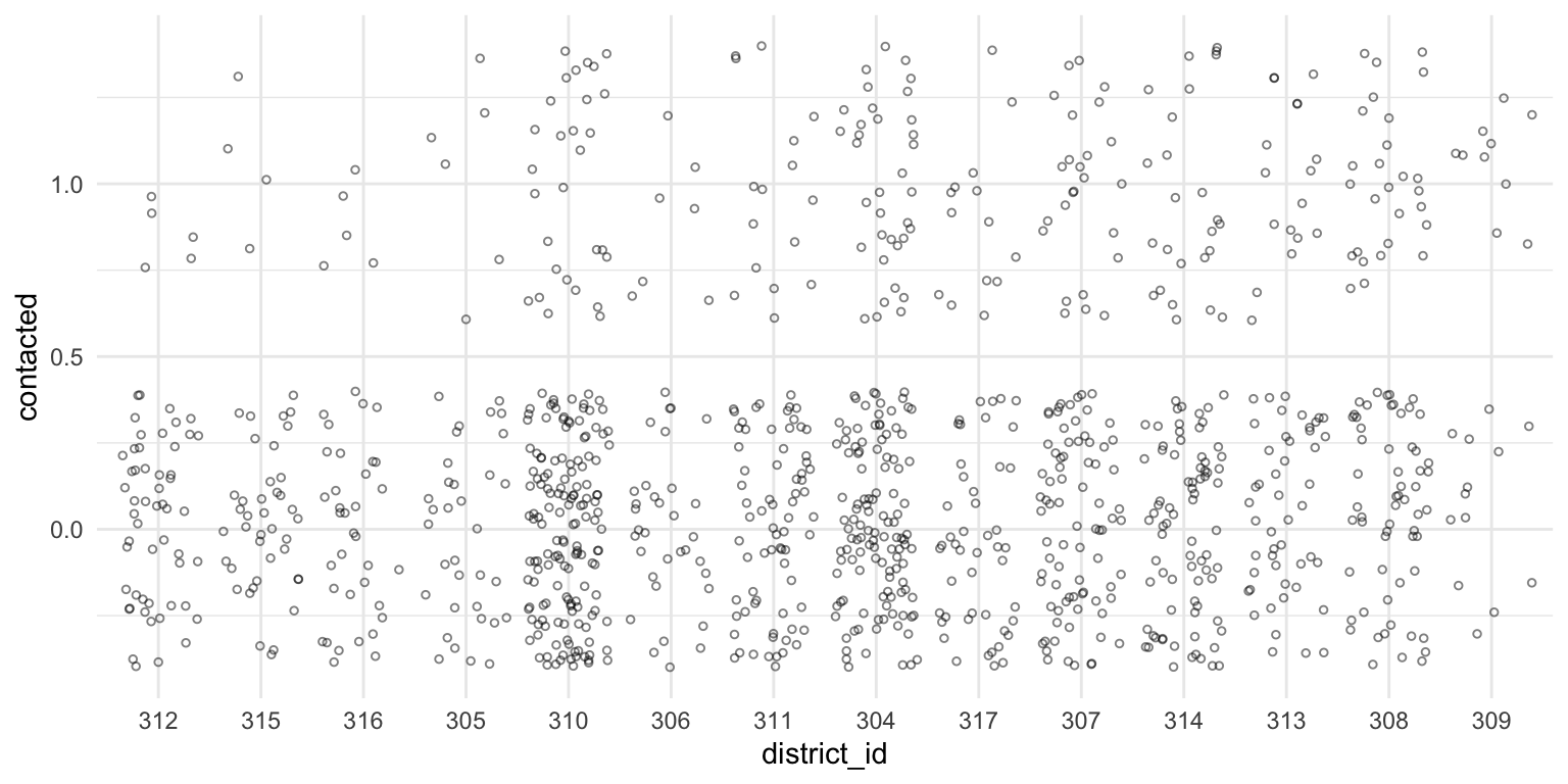
Here are the packages we’re using:
This week, I introduce the idea of a hierarchical model.
These fall squarely within our probability modeling framework—but with an exciting new twist.
Before: \(x_i \sim f(x_i; \theta)\)
Now: \(x_i \sim f(x_i; \theta_{j[i]})\), where \(\theta_j \sim f(\theta_j; \phi)\)
We have models of parameters \(\theta_j \sim f(\theta_j; \phi)\) analogous to a previous models of data.
In my dissertation, I was interested in how survey self-reports of being contacted by a political party varies across electoral districts.
You can see here for the details.
finland dataFor now, let’s just estimate the proportion of people in each district that are contacted by a party.
Let’s start with Finland.
Rows: 1,086
Columns: 2
$ district_id <chr> "District 313", "District 313", "District 310", "District 304", "Dis…
$ contacted <fct> Not Contacted, Contacted, Not Contacted, Contacted, Not Contacted, N…
It will be convenient in later steps to have contacted be an indicator and district_id be a nice factor, so let’s do that now.
reorder() the levels by the average of contacted. (Important sneaky trick).finland data, tidied up# load data
finland <- crdata::finland |>
# make contacted an indicator
mutate(contacted = as.numeric(contacted == "Contacted")) |>
# mutate district_id to factor ordered by contact rate
mutate(district_id = str_remove(district_id, "District "),
district_id = reorder(district_id, contacted)) |>
glimpse()Rows: 1,086
Columns: 2
$ district_id <fct> 313, 313, 310, 304, 304, 304, 304, 304, 304, 304, 304, 304, 304, 304…
$ contacted <dbl> 0, 1, 0, 1, 0, 0, 0, 1, 0, 0, 0, 0, 0, 1, 0, 1, 1, 0, 0, 1, 1, 0, 0,…
A scatterplot is a safe and potentially informative way to start.
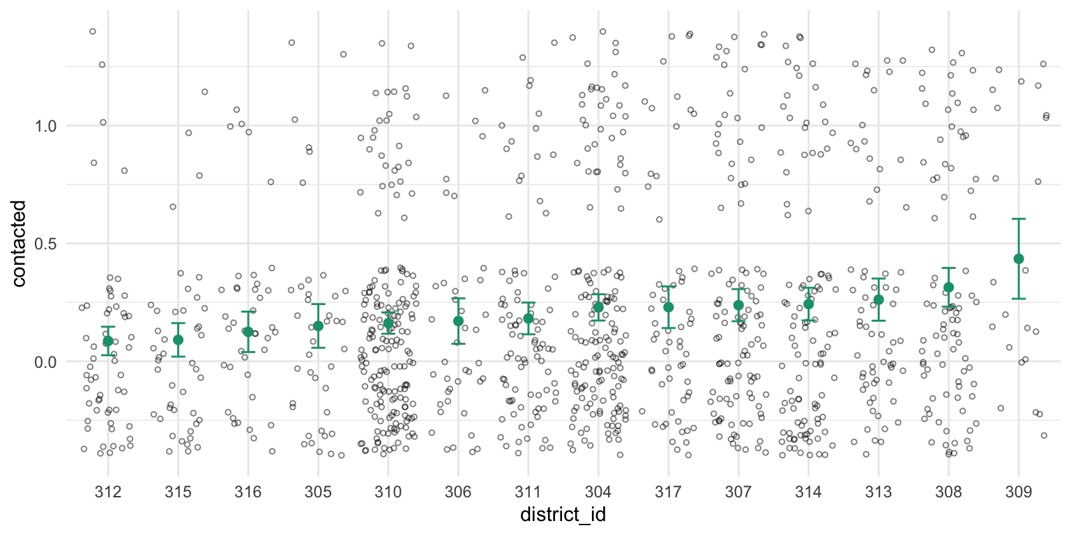
Now let’s estimate the probability of being contacted by a political party in each district.
Start by writing down a probability model for being contacted. This is a binary outcome, so if we’re going to assume (conditional) independence, it must be Bernoulli.
\[ \text{Contacted}_i \sim \text{Bernoulli}(\pi_j), \]
where \(i\) indexes the respondent and \(j\) indexes the electoral district.
Remember that the ML estimate of \(\pi\) is just the sample mean (or sample proportion).
We can do this easily for each district with group_by() and summarize().
Let’s also add an estimate of the standard error using \(\widehat{\text{SE}}(\hat{\pi}_j) = \frac{\sqrt{\hat{\pi}_j(1 - \hat{\pi}_j)}}{\sqrt{n}}\).
estimates <- finland %>%
group_by(district_id) %>%
summarize(pi_hat = mean(contacted),
n = n(),
se_hat = sqrt(pi_hat*(1 - pi_hat))/sqrt(n)) %>%
glimpse()Rows: 14
Columns: 4
$ district_id <fct> 312, 315, 316, 305, 310, 306, 311, 304, 317, 307, 314, 313, 308, 309
$ pi_hat <dbl> 0.0862, 0.0909, 0.1250, 0.1500, 0.1620, 0.1707, 0.1818, 0.2288, 0.22…
$ n <int> 58, 44, 40, 40, 179, 41, 88, 153, 61, 105, 103, 65, 86, 23
$ se_hat <dbl> 0.0369, 0.0433, 0.0523, 0.0565, 0.0275, 0.0588, 0.0411, 0.0340, 0.05…
Now let’s add these estimates to the scatterplot.
You can see that the confidence intervals (and sample size) varies by district, so let’s add that information to the plot.
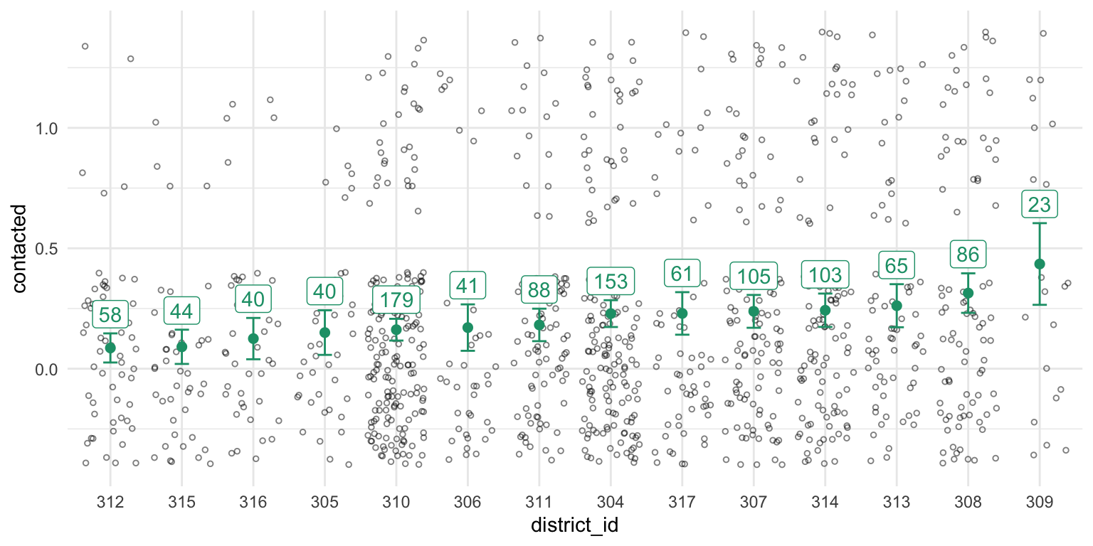
Great! Now we’re done. We’ve got ML estimates of the contact rate for all districts.
But wait… can we do better?
Let’s look at district 309 on the far right. We our estimate of the contact rate in this district is the highest.
Our estimator \(\hat\pi\) is unbiased, but if you had to say, would you say that the turnout rate in district 309 was higher or lower than \(\hat{\pi}_{309} = 0.40\)?
If your intuition matches mine, you will say lower. Why? This “why?” is an important question.
This is exactly the intuition of hierarchical models.
Let’s write down this “different, but similar” intuition.
To do this, it will be convenient to have our \(\pi_j\)s on the logit scale.
Start with the likelihood.
\[ \text{Contacted}_i \sim \text{Bernoulli}(\pi_j) \]
Now translate the \(\pi\)s to the logit scale.
\[ \pi_j = \text{logit}^{-1}(\alpha_j) \]
Each of these \(\alpha_j\)s is like a constant term in a logit model with no covariates. (We could add covariates, but that makes the example less clear.)
Now for the hierarchical part: we want to capture the notion that these \(\alpha_j\)s are different but similar.
We can do that by modeling them as draws from normal distribution.
\[ \alpha_j \sim N(\mu, \sigma^2) \]
We can estimate \(\mu\) (the “typical” \(\alpha\)) and \(\sigma\) (the degree of similarity) from the data. This is “hierarchical piece.”
We sometimes refer to batches of parameters modeled as draws from a distribution as “random effects.”
To estimate the hierarchical model:
lme4::lmer()/lme4::glmer() function. Fast, fragile, approximate.brm() function. Slow(er), robust, exact.1We’re going to start with lmer() because I don’t want to juggle posterior simulation and hierarchical models simultaneously, but you should always use brm() (or Stan some other way) always unless you simply need a quick fit.
lmer()We can fit the model with glmer().
And we can summarize the results.
glmer(formula = contacted ~ (1 | district_id), data = finland,
family = binomial)
coef.est coef.se
-1.37 0.12
Error terms:
Groups Name Std.Dev.
district_id (Intercept) 0.31
Residual 1.00
---
number of obs: 1086, groups: district_id, 14
AIC = 1108.5, DIC = 1070
deviance = 1087.0
From the output above, we estimate \(\mu\) as -1.37 and \(\sigma\) as 0.31. That is, the \(\alpha_j\)s are about -1.37 give-or-take 0.31 or so.
group-level effects 👉 “random effects”
But here’s the useful part: we can take this \(\hat{\mu}\) and \(\hat{\sigma}\) and use them as a Bayesian prior for the individual \(\alpha_j\)s.
Each \(\alpha_j\) has a likelihood (using the data from that district) and a prior (using \(\hat{\mu}\) and \(\hat{\sigma}\)).
(Intercept)
-1.37
# (alpha - mu)
# - random part
# - deviation from the typical intercept for each district
re <- ranef(fit)$district_id[, "(Intercept)"] # ️👈 "random effects"‼️
re [1] -0.3586 -0.2901 -0.1875 -0.1260 -0.1917 -0.0768 -0.0743 0.1125 0.0809 0.1339
[11] 0.1497 0.1793 0.3718 0.3681
[1] -1.73 -1.66 -1.56 -1.50 -1.56 -1.45 -1.45 -1.26 -1.29 -1.24 -1.22 -1.19 -1.00 -1.00
[1] 0.151 0.160 0.174 0.183 0.173 0.190 0.191 0.221 0.216 0.225 0.228 0.233 0.269 0.268
predict()In this case, it’s easy to use predict() to get this same estimates. (The predict() approach is a little safer because it’s easier to keep the pi_hat and the district_id label together.)
hier_estimates <- tibble(district_id = unique(finland$district_id)) %>%
mutate(pi_hat = predict(fit, newdata = ., type = "response")) %>%
arrange(district_id) %>%
glimpse()Rows: 14
Columns: 2
$ district_id <fct> 312, 315, 316, 305, 310, 306, 311, 304, 317, 307, 314, 313, 308, 309
$ pi_hat <dbl> 0.151, 0.160, 0.174, 0.183, 0.173, 0.190, 0.191, 0.221, 0.216, 0.225…
We can also do this with {marginaleffects}.
predictions(fit,
newdata = datagrid(district_id = unique)) |>
select(district_id, estimate) |>
arrange(district_id) |> # comparisons() arranges predictions differently
glimpse()Rows: 14
Columns: 2
$ district_id <fct> 312, 315, 316, 305, 310, 306, 311, 304, 317, 307, 314, 313, 308, 309
$ estimate <dbl> 0.151, 0.160, 0.174, 0.183, 0.173, 0.190, 0.191, 0.221, 0.216, 0.225…
We can add this to our plot to see how the estimates changed.
We can compare the initial ML estimates to the hierarchical model estimates.
Rows: 28
Columns: 5
$ type <chr> "initial ML", "initial ML", "initial ML", "initial ML", "initial ML"…
$ district_id <fct> 312, 315, 316, 305, 310, 306, 311, 304, 317, 307, 314, 313, 308, 309…
$ pi_hat <dbl> 0.0862, 0.0909, 0.1250, 0.1500, 0.1620, 0.1707, 0.1818, 0.2288, 0.22…
$ n <int> 58, 44, 40, 40, 179, 41, 88, 153, 61, 105, 103, 65, 86, 23, NA, NA, …
$ se_hat <dbl> 0.0369, 0.0433, 0.0523, 0.0565, 0.0275, 0.0588, 0.0411, 0.0340, 0.05…
It’s helpful to think of these approaches in terms of the amount of information they borrow across groups.
We did not implement complete pooling above, but we can do it here to compare the three approaches.
# use the overall rate for each district
common_estimate <- tibble(district_id = unique(finland$district_id)) %>%
mutate(pi_hat = mean(finland$contacted))
# combine the three types
comb <- bind_rows(list("No Pooling" = estimates,
"Partial Pooling" = hier_estimates,
"Complete Pooling" = common_estimate),
.id = "type") %>%
mutate(type = reorder(type, pi_hat, var))
gg_comb2 <- ggplot(comb, aes(x = pi_hat, y = type)) +
geom_point(alpha = 0.5) +
geom_line(aes(group = district_id), alpha = 0.5)
print(gg_comb2) First, the 309 problem.
Second, \(\mu_i = \alpha_{j[i]} + \beta x_i\), where \(\alpha_j \sim N(0, \sigma^2_\alpha)\).
Third, the figure below.
uk <- crdata::uk |>
# make contacted an indicator
mutate(contacted = as.numeric(contacted == "Contacted")) |>
# mutate district_id to factor ordered by contact rate
mutate(district_id = str_remove(district_id, "District "),
district_id = reorder(district_id, contacted)) |>
glimpse()Rows: 756
Columns: 3
$ district_id <fct> 492, 492, 492, 492, 492, 374, 350, 350, 350, 463, 463, …
$ contacted <dbl> 0, 0, 0, 0, 0, 0, 1, 0, 0, 0, 0, 1, 0, 0, 0, 0, 0, 0, 1…
$ district_competitiveness <dbl> 0.484, 0.484, 0.484, 0.484, 0.484, 0.510, 0.540, 0.540,…
estimates <- uk %>%
group_by(district_id) %>%
summarize(pi_hat = mean(contacted),
n = n(),
se_hat = sqrt(pi_hat*(1 - pi_hat))/sqrt(n)) %>%
glimpse()Rows: 253
Columns: 4
$ district_id <fct> 319, 320, 323, 326, 328, 329, 330, 331, 337, 338, 339, 344, 347, 348…
$ pi_hat <dbl> 0, 0, 0, 0, 0, 0, 0, 0, 0, 0, 0, 0, 0, 0, 0, 0, 0, 0, 0, 0, 0, 0, 0,…
$ n <int> 1, 2, 4, 2, 3, 2, 2, 1, 4, 1, 1, 2, 2, 1, 1, 1, 2, 2, 6, 4, 1, 3, 1,…
$ se_hat <dbl> 0, 0, 0, 0, 0, 0, 0, 0, 0, 0, 0, 0, 0, 0, 0, 0, 0, 0, 0, 0, 0, 0, 0,…
complete_pooling <- tibble(district_id = unique(uk$district_id)) %>%
mutate(pi_hat = mean(uk$contacted)) %>%
glimpse()Rows: 253
Columns: 2
$ district_id <fct> 492, 374, 350, 463, 393, 366, 432, 375, 385, 377, 378, 461, 387, 367…
$ pi_hat <dbl> 0.32, 0.32, 0.32, 0.32, 0.32, 0.32, 0.32, 0.32, 0.32, 0.32, 0.32, 0.…
glmer(formula = contacted ~ (1 | district_id), data = uk, family = binomial)
coef.est coef.se
-0.85 0.10
Error terms:
Groups Name Std.Dev.
district_id (Intercept) 0.71
Residual 1.00
---
number of obs: 756, groups: district_id, 253
AIC = 941.8, DIC = 694
deviance = 815.8
partial_pooling <- tibble(district_id = unique(uk$district_id)) %>%
mutate(pi_hat = predict(fit, newdata = ., type = "response")) %>%
arrange(district_id) %>%
glimpse()Rows: 253
Columns: 2
$ district_id <fct> 319, 320, 323, 326, 328, 329, 330, 331, 337, 338, 339, 344, 347, 348…
$ pi_hat <dbl> 0.271, 0.249, 0.216, 0.249, 0.231, 0.249, 0.249, 0.271, 0.216, 0.271…
comb <- bind_rows(list("No Pooling" = no_pooling,
"Partial Pooling" = partial_pooling,
"Complete Pooling" = complete_pooling),
.id = "type") %>%
mutate(type = reorder(type, pi_hat, var)) %>%
arrange(district_id) %>%
glimpse()Rows: 759
Columns: 3
$ type <fct> No Pooling, Partial Pooling, Complete Pooling, No Pooling, Partial P…
$ district_id <fct> 319, 319, 319, 320, 320, 320, 323, 323, 323, 326, 326, 326, 328, 328…
$ pi_hat <dbl> 0.000, 0.271, 0.320, 0.000, 0.249, 0.320, 0.000, 0.216, 0.320, 0.000…
We can also add predictors of the random parameters, such as the competitiveness of the district.
Rows: 253
Columns: 2
$ district_id <fct> 492, 374, 350, 463, 393, 366, 432, 375, 385, 377, 378, …
$ district_competitiveness <dbl> 0.484, 0.510, 0.540, 0.454, 0.429, 0.676, 0.603, 0.588,…
Rows: 253
Columns: 3
$ district_id <fct> 319, 320, 323, 326, 328, 329, 330, 331, 337, 338, 339, …
$ pi_hat <dbl> 0.271, 0.249, 0.216, 0.249, 0.231, 0.249, 0.249, 0.271,…
$ district_competitiveness <dbl> 0.584, 0.658, 0.657, 0.453, 0.676, 0.686, 0.659, 0.679,…
Hey! We should build this directly into our model.
f <- contacted ~ district_competitiveness + (1 | district_id)
fit <- glmer(f, data = uk, family = binomial)
arm::display(fit)glmer(formula = contacted ~ district_competitiveness + (1 | district_id),
data = uk, family = binomial)
coef.est coef.se
(Intercept) -3.40 0.65
district_competitiveness 3.87 0.96
Error terms:
Groups Name Std.Dev.
district_id (Intercept) 0.60
Residual 1.00
---
number of obs: 756, groups: district_id, 253
AIC = 927.2, DIC = 740
deviance = 830.5
partial_pooling <- uk %>%
select(district_id, district_competitiveness) %>%
distinct() %>%
mutate(pi_hat = predict(fit, newdata = ., type = "response")) %>%
glimpse()Rows: 253
Columns: 3
$ district_id <fct> 492, 374, 350, 463, 393, 366, 432, 375, 385, 377, 378, …
$ district_competitiveness <dbl> 0.484, 0.510, 0.540, 0.454, 0.429, 0.676, 0.603, 0.588,…
$ pi_hat <dbl> 0.144, 0.183, 0.230, 0.185, 0.137, 0.303, 0.204, 0.258,…
comb <- bind_rows(list("No Pooling" = no_pooling,
"Partial Pooling" = partial_pooling,
"Complete Pooling" = complete_pooling),
.id = "type") %>%
mutate(type = reorder(type, pi_hat, var)) %>%
glimpse()Rows: 759
Columns: 4
$ type <fct> No Pooling, No Pooling, No Pooling, No Pooling, No Pool…
$ district_id <fct> 319, 320, 323, 326, 328, 329, 330, 331, 337, 338, 339, …
$ pi_hat <dbl> 0, 0, 0, 0, 0, 0, 0, 0, 0, 0, 0, 0, 0, 0, 0, 0, 0, 0, 0…
$ district_competitiveness <dbl> NA, NA, NA, NA, NA, NA, NA, NA, NA, NA, NA, NA, NA, NA,…
\[ \text{Pr}(\text{Contacted}_{i} = 1) = \text{logit}^{-1}(\alpha_{jk} + {\bf X}_i\beta) \] \[ \alpha_{jk} \sim N(\gamma_{0k} + \gamma_{1k}\text{Competitiveness}_j, \sigma^2_{\alpha}) \text{ for } j = 1, 2,..., J \]
\[ \begin{pmatrix} \gamma_{0k} \\ \gamma_{1k} \end{pmatrix} \sim {\large} N\begin{pmatrix} \begin{pmatrix} \mu_{\gamma_{0}} \\ \mu_{\gamma_{1}} \end{pmatrix}, \begin{pmatrix} \sigma^2_{\gamma_{0}} & \rho\sigma_{\gamma_{0}}\sigma_{\gamma_{1}} \\ \rho\sigma_{\gamma_{0}}\sigma_{\gamma_{1}} & \sigma^2_{\gamma_{1}} \end{pmatrix}\end{pmatrix} \text{ , for }k = 1, 2, ..., K \]
\[ \mu_{\gamma_{0}} = \delta_{00} + \delta_{01}\text{Proportional Rules}_k \]
\[ \mu_{\gamma_{1}} = \delta_{10} + \delta_{11}\text{Proportional Rules}_k \]
Rows: 5,126
Columns: 5
$ election_id <chr> "Canada", "Canada", "Canada", "Canada", "Canada", "Cana…
$ district_id <chr> "Canada; District 7", "Canada; District 4", "Canada; Di…
$ contacted <fct> Contacted, Not Contacted, Not Contacted, Not Contacted,…
$ district_competitiveness <dbl> 0.740, 0.420, 0.692, 0.692, 0.610, 0.742, 0.742, 0.742,…
$ electoral_rules <fct> SMD, SMD, SMD, SMD, SMD, SMD, SMD, SMD, SMD, SMD, SMD, …
We can fit this model with lmer(), but this relatively small model is too big or complex.
Stan would have no problems with this one…
And show the estimates.
glmer(formula = contacted ~ district_competitiveness * electoral_rules +
(1 | district_id) + (1 + district_competitiveness | election_id),
data = rainey, family = binomial)
coef.est coef.se z value Pr(>|z|)
(Intercept) -2.35 0.59 -4.01 0.00
district_competitiveness 1.21 0.81 1.49 0.14
electoral_rulesSMD -0.74 0.72 -1.03 0.30
district_competitiveness:electoral_rulesSMD 3.07 1.03 2.99 0.00
Error terms:
Groups Name Std.Dev. Corr
district_id (Intercept) 0.47
election_id (Intercept) 0.18
district_competitiveness 0.27 1.00
Residual 1.00
---
number of obs: 5126, groups: district_id, 567; election_id, 5
AIC = 5580.3, DIC = 5131
deviance = 5347.5
Using the lmer()-like formula, we can fit the hiearchical model with Stan.
And it fits in less than 10 minutes. This took hours or days in 2012 with JAGS.
Family: bernoulli
Links: mu = logit
Formula: contacted ~ district_competitiveness * electoral_rules + (1 | district_id) + (1 + district_competitiveness | election_id)
Data: rainey (Number of observations: 5126)
Draws: 10 chains, each with iter = 4000; warmup = 2000; thin = 1;
total post-warmup draws = 20000
Multilevel Hyperparameters:
~district_id (Number of levels: 567)
Estimate Est.Error l-95% CI u-95% CI Rhat Bulk_ESS Tail_ESS
sd(Intercept) 0.52 0.08 0.38 0.69 1.01 2641 4441
~election_id (Number of levels: 5)
Estimate Est.Error l-95% CI u-95% CI Rhat
sd(Intercept) 0.64 0.51 0.03 1.97 1.01
sd(district_competitiveness) 1.00 0.91 0.04 3.28 1.04
cor(Intercept,district_competitiveness) -0.06 0.57 -0.94 0.95 1.01
Bulk_ESS Tail_ESS
sd(Intercept) 2851 3648
sd(district_competitiveness) 173 49
cor(Intercept,district_competitiveness) 1752 5597
Regression Coefficients:
Estimate Est.Error l-95% CI u-95% CI Rhat
Intercept -2.39 0.76 -3.88 -0.88 1.01
district_competitiveness 1.41 1.16 -0.69 4.05 1.04
electoral_rulesSMD -0.74 1.02 -2.84 1.25 1.01
district_competitiveness:electoral_rulesSMD 3.09 1.57 0.01 6.58 1.05
Bulk_ESS Tail_ESS
Intercept 2798 4956
district_competitiveness 190 118
electoral_rulesSMD 2102 1009
district_competitiveness:electoral_rulesSMD 126 35
Draws were sampled using sample(hmc). For each parameter, Bulk_ESS
and Tail_ESS are effective sample size measures, and Rhat is the potential
scale reduction factor on split chains (at convergence, Rhat = 1).
grid <- rainey %>%
select(district_id,
election_id,
district_competitiveness,
electoral_rules)
p <- predictions(stan_fit,
newdata = grid) |>
glimpse()Rows: 5,126
Columns: 9
$ rowid <int> 1, 2, 3, 4, 5, 6, 7, 8, 9, 10, 11, 12, 13, 14, 15, 16, …
$ estimate <dbl> 0.695, 0.312, 0.567, 0.567, 0.568, 0.629, 0.629, 0.629,…
$ conf.low <dbl> 0.465, 0.144, 0.324, 0.324, 0.319, 0.402, 0.402, 0.402,…
$ conf.high <dbl> 0.865, 0.560, 0.773, 0.773, 0.784, 0.815, 0.815, 0.815,…
$ district_id <chr> "Canada; District 7", "Canada; District 4", "Canada; Di…
$ election_id <chr> "Canada", "Canada", "Canada", "Canada", "Canada", "Cana…
$ district_competitiveness <dbl> 0.740, 0.420, 0.692, 0.692, 0.610, 0.742, 0.742, 0.742,…
$ electoral_rules <fct> SMD, SMD, SMD, SMD, SMD, SMD, SMD, SMD, SMD, SMD, SMD, …
$ df <dbl> Inf, Inf, Inf, Inf, Inf, Inf, Inf, Inf, Inf, Inf, Inf, …
p_typical <- predictions(
stan_fit,
newdata = grid,
re_formula = ~ (1 + district_competitiveness | election_id)
) |>
glimpse()Rows: 5,126
Columns: 9
$ rowid <int> 1, 2, 3, 4, 5, 6, 7, 8, 9, 10, 11, 12, 13, 14, 15, 16, …
$ estimate <dbl> 0.660, 0.296, 0.606, 0.606, 0.510, 0.662, 0.662, 0.662,…
$ conf.low <dbl> 0.605, 0.227, 0.558, 0.558, 0.465, 0.607, 0.607, 0.607,…
$ conf.high <dbl> 0.711, 0.375, 0.653, 0.653, 0.556, 0.713, 0.713, 0.713,…
$ district_id <chr> "Canada; District 7", "Canada; District 4", "Canada; Di…
$ election_id <chr> "Canada", "Canada", "Canada", "Canada", "Canada", "Cana…
$ district_competitiveness <dbl> 0.740, 0.420, 0.692, 0.692, 0.610, 0.742, 0.742, 0.742,…
$ electoral_rules <fct> SMD, SMD, SMD, SMD, SMD, SMD, SMD, SMD, SMD, SMD, SMD, …
$ df <dbl> Inf, Inf, Inf, Inf, Inf, Inf, Inf, Inf, Inf, Inf, Inf, …