Multinomial Logit

The Inverse-Logit Function

Suppose \(y_i \in \{0, 1\}\). Using logistic regression, we model \(\Pr(y_i = 1)\) as a function of covariates, so that

\[ \Pr(Y_i = 1) = \frac{\exp(X_i \beta)}{1 + \exp(X_i \beta)}. \]

The function \(f(z) = \frac{e^z}{1 + e^z}\) is called the inverse-logit function and maps any real number \(X_i \beta\) into a probability between 0 and 1.

Because the two probabilities must sum to one:

\[ \Pr(Y_i = 0) = 1 - \Pr(Y_i = 1) = \frac{1}{1 + \exp(X_i \beta)}. \]

The Softmax Function

The softmax generalizes the inverse-logit—it takes \(J\) real inputs (i.e., from \(\mathbb{R}^J\)) and scales them to sum to one.

\[ \text{softmax}(z_j) = \frac{\exp(z_j)}{\sum_{k=1}^{J} \exp(z_k)}, \qquad j = 1,\ldots,J. \] Because the \(J\) outputs must sum to one, it is natural to interpret the outputs as probabilities.

The OJS widget below allows you to experiment with \(J = 4\) inputs and see how the outputted probabilities change.

viewof z1 = Inputs.range([-5, 5], {step: 0.1, value: 1,   label: "z1"});
viewof z2 = Inputs.range([-5, 5], {step: 0.1, value: 0.5, label: "z2"});
viewof z3 = Inputs.range([-5, 5], {step: 0.1, value: -0.5,label: "z3"});
viewof z4 = Inputs.range([-5, 5], {step: 0.1, value: -1,  label: "z4"});

// Softmax pieces
labels = ["Pr(A)","Pr(B)","Pr(C)","Pr(D)"];
zs = [z1, z2, z3, z4];
exps = zs.map(Math.exp);
sumexp = exps.reduce((a, b) => a + b, 0);
ps = exps.map(e => e / sumexp);

// Data for stacked bar (one row, four segments)
data = ps.map((p, i) => ({ label: labels[i], value: p, row: "softmax" }));

// === Two-column layout: sliders (left) + live table (right) ===
{
const container = html`<div style="
  display:flex;
  gap:24px;
  align-items:flex-start;
  padding-top:8px;
"></div>`;

// Left column: sliders
const left = html`<div style="display:grid; gap:10px; min-width:220px;"></div>`;
left.append(viewof z1, viewof z2, viewof z3, viewof z4);

// Right column: table
const rows = labels.map((cls, i) => ({
Class: cls,
z: zs[i],
"exp(z)": exps[i],
Probability: ps[i]
}));

const right = html`<div style="
  min-width:240px;
  max-width:660px;
  padding:4px 0;
  font-size:2.00rem;
  line-height:1.1;
"></div>`;

right.append(
Inputs.table(rows, {
columns: ["Class", "z", "exp(z)", "Probability"],
format: {
z: d => d.toFixed(2),
"exp(z)": d => d.toFixed(3),
Probability: d => (d * 100).toFixed(1) + "%"
}
})
);

container.append(left, right);
return container;
}

Plot.plot({
width: 900,              // wider
height: 120,             // taller
marginLeft: 20,
marginRight: 20,
marginBottom: 50,
x: {
domain: [0, 1],
tickFormat: d => (d * 100).toFixed(0) + "%",
label: "Probability",
labelArrow: false,
labelAnchor: "center",
tickSize: 10,
tickPadding: 8
},
y: { axis: null },

// Bigger fonts everywhere
style: {
fontSize: "18px",        // main text size
fontFamily: "sans-serif"
},

color: {
legend: true,
label: "Class",
tickSize: 12
},

marks: [
Plot.barX(
data,
Plot.stackX({ x: "value", y: "row", fill: "label", sort: { fill: null } })
),
Plot.ruleX([0, 1])
]
})

Adding covariates

Now suppose the outcome takes \(J\) possible values:

\[ y_i \in \{1, 2, \ldots, J\}. \]

Example 1: We might label vote choice in the US as (1) abstain, (2) Republican, (3) Democrat, or (4) other.

Example 2: We might label coup attempts in a given country-year as (0) none attempted, (1) failed attempt, or (2) successful attempt.

For each category \(j\), define a linear predictor \(\eta_{ij} = X_i \beta_j\). Here, each \(\beta_j\) is a vector of coefficients.

We can use the softmax function to convert these linear predictors into probabilities that sum to one.

\[ \Pr(Y_i = j) = \frac{\exp(\eta_{ij})}{\sum_{k=1}^{J} \exp(\eta_{ik})}, \qquad j = 1, \ldots, J. \]

This is a generalization of the inverse-logit to \(J\) categories. If \(J = 2\), the softmax reduces to the inverse-logit.

However, this model is not identified because adding any constant to each of the \(\eta_{ij}\) produces the same probabilities.

Example Inputs

Input \(z_j\)	Softmax \(p_j\)
\(-1\)	0.0303
\(1\)	0.2242
\(2\)	0.6095
\(0.5\)	0.1360

Adding a Constant (\(+2\))

New Input \(z_j + 2\)	Softmax \(p_j\)
\(-1 + 2 = 1\)	0.0303
\(1 + 2 = 3\)	0.2242
\(2 + 2 = 4\)	0.6095
\(0.5 + 2 = 2.5\)	0.1360

Adding a constant to all inputs leaves the softmax unchanged. This is why the multinomial logit model requires an identification constraint.

To identify the model, we set \(\beta_J = 0\), so that \(\eta_{iJ} = 0\). Then for \(j = 1, \ldots, J-1\), we have

\[ \Pr(Y_i = j) = \frac{\exp(X_i \beta_j)} {1 + \sum_{k=1}^{J-1} \exp(X_i \beta_k)}. \]

And for the “baseline” category \(J\), we have

\[ \Pr(Y_i = J) = \frac{1} {1 + \sum_{k=1}^{J-1} \exp(X_i \beta_k)}. \]

Example: The 1992 presidential vote

Data

• 1992 ANES (Miller et al. 2016); same respondents as the wk06 Bush approval example
• Outcome: vote_1992: Bush, Clinton, or Perot
• Predictors: party_id (−3 to 3), economy (1 = much better to 5 = much worse)
• [CTK: why Perot makes this nominal, not ordered]

# load data; keep complete cases on the model's variables
vote <- read_csv("https://pos5747.github.io/data/bush-approval-1992.csv") |>
  select(vote_1992, party_id, economy) |>
  drop_na() |>
  mutate(vote_1992 = factor(vote_1992, levels = c("Bush", "Clinton", "Perot"))) |>
  glimpse()

Rows: 592
Columns: 3
$ vote_1992 <fct> Bush, Bush, Bush, Clinton, Clinton, Clinton, Bush, Bush, Bus…
$ party_id  <dbl> 2, 3, 3, 3, -2, -3, 2, 3, 2, 1, -3, -2, 3, 1, -1, -3, -1, -3…
$ economy   <dbl> 4, 4, 3, 3, 5, 5, 4, 2, 4, 3, 5, 4, 4, 4, 5, 5, 4, 5, 4, 5, …

multinom()

library(nnet)  # for multinom()

# fit multinomial logit; first level (Bush) is the baseline
fit_vote <- multinom(vote_1992 ~ party_id + economy, data = vote, trace = FALSE)
summary(fit_vote)

Call:
multinom(formula = vote_1992 ~ party_id + economy, data = vote, 
    trace = FALSE)

Coefficients:
        (Intercept)   party_id   economy
Clinton   -1.977521 -1.0977031 0.5514930
Perot     -1.518696 -0.4389651 0.3361671

Std. Errors:
        (Intercept)   party_id   economy
Clinton   0.6221333 0.08564888 0.1512617
Perot     0.5848327 0.07740859 0.1437105

Residual Deviance: 869.9068 
AIC: 881.9068 

• [CTK: one row of coefficients per non-baseline candidate, each relative to Bush]

Probabilities with {marginaleffects}

library(marginaleffects)

# probability of each candidate as party ID varies
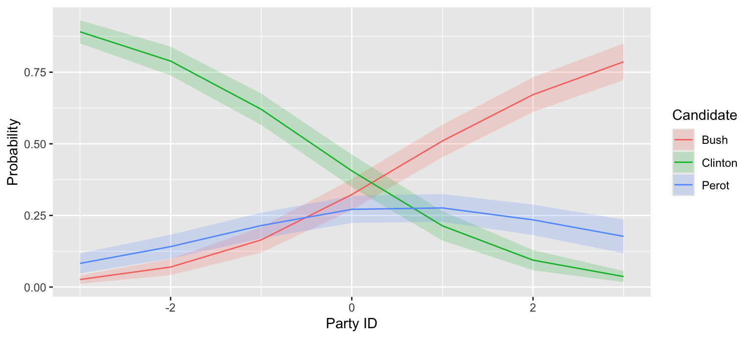
p <- predictions(fit_vote, newdata = datagrid(party_id = -3:3), type = "probs")

# A tibble: 7 × 4
  party_id  Bush Clinton Perot
     <int> <dbl>   <dbl> <dbl>
1       -3  0.03    0.89  0.08
2       -2  0.07    0.79  0.14
3       -1  0.16    0.62  0.21
4        0  0.32    0.41  0.27
5        1  0.51    0.21  0.28
6        2  0.67    0.09  0.23
7        3  0.79    0.04  0.18

Probabilities with {marginaleffects}

ggplot(p, aes(x = party_id, y = estimate, ymin = conf.low, ymax = conf.high,
              color = group, fill = group)) +
  geom_ribbon(alpha = 0.2, color = NA) +
  geom_line() +
  labs(x = "Party ID", y = "Probability", color = "Candidate", fill = "Candidate")

• [CTK: Pr(Perot) rises then falls, though both linear predictors are linear in party ID]

First differences

# change in each candidate's probability as the economy goes from 2 to 4
comparisons(fit_vote,
            variables = list(economy = c(2, 4)),
            newdata = datagrid(grid_type = "mean_or_mode"),
            type = "probs")

   Group Estimate Std. Error      z Pr(>|z|)    S   2.5 %  97.5 %
 Bush     -0.2188     0.0628 -3.487   <0.001 11.0 -0.3418 -0.0958
 Clinton   0.1799     0.0472  3.811   <0.001 12.8  0.0874  0.2724
 Perot     0.0389     0.0458  0.851    0.395  1.3 -0.0508  0.1287

Term: economy
Type: probs
Comparison: 4 - 2

• [CTK: Perot’s economy coefficient is positive, but Clinton gains most of what Bush loses]

brm()

library(brms)

# categorical() is the multinomial logit; first level (Bush) is the baseline
fit_vote_brm <- brm(vote_1992 ~ party_id + economy,
                    data = vote,
                    family = categorical(link = "logit"),
                    backend = "cmdstanr",
                    chains = 4,
                    cores = 4,
                    seed = 1234)

brm() vs. multinom()

# posterior means next to the ML estimates
fixef(fit_vote_brm)[, c("Estimate", "Q2.5", "Q97.5")]

                      Estimate        Q2.5      Q97.5
muClinton_Intercept -1.9872399 -3.20025522 -0.7418053
muPerot_Intercept   -1.5388153 -2.75225907 -0.4053306
muClinton_party_id  -1.1118213 -1.28144202 -0.9499521
muClinton_economy    0.5540187  0.25335790  0.8462712
muPerot_party_id    -0.4453109 -0.59737345 -0.2927705
muPerot_economy      0.3408766  0.05805077  0.6306184

coef(fit_vote)

        (Intercept)   party_id   economy
Clinton   -1.977521 -1.0977031 0.5514930
Perot     -1.518696 -0.4389651 0.3361671

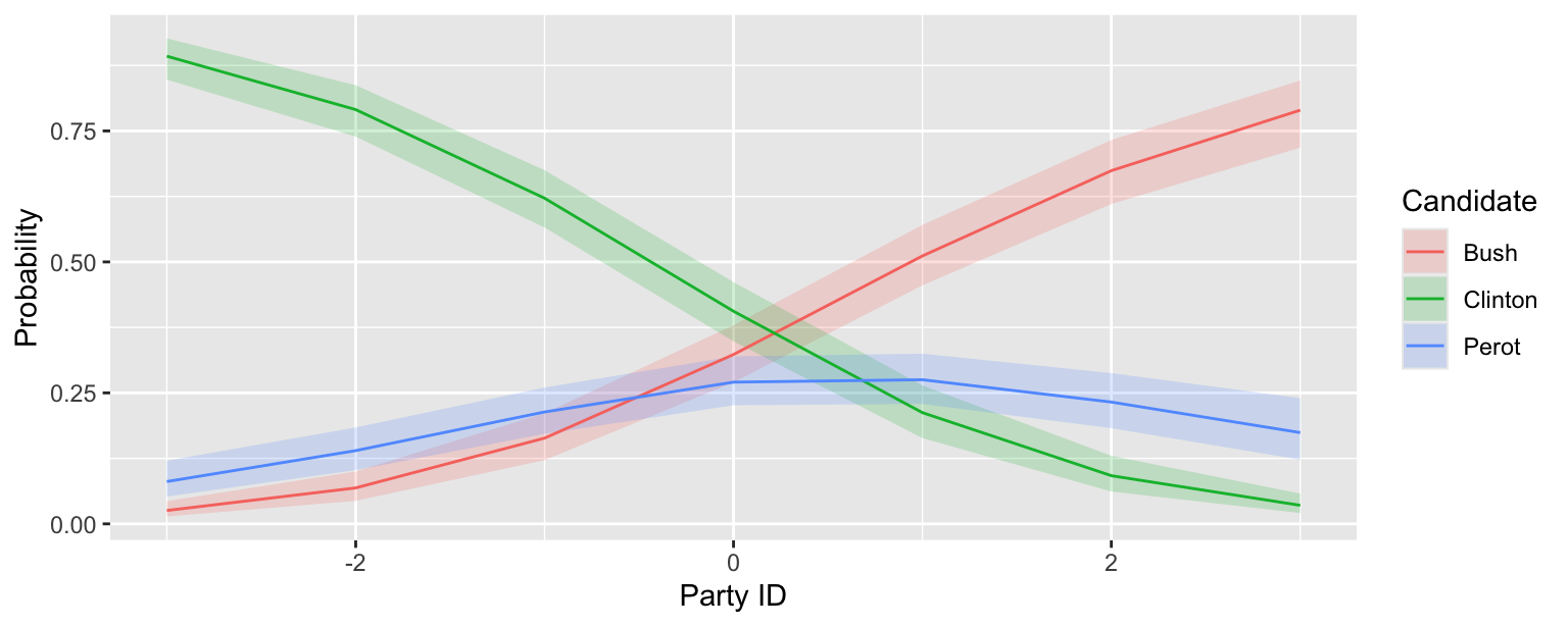
brm() + {marginaleffects}

# predictions() returns rowid but not the grid columns for this fit, so join them back
grid <- datagrid(model = fit_vote_brm, party_id = -3:3)
p_brm <- predictions(fit_vote_brm, newdata = grid) |>
  left_join(select(grid, rowid, party_id), by = "rowid")

ggplot(p_brm, aes(x = party_id, y = estimate, ymin = conf.low, ymax = conf.high,
                  color = group, fill = group)) +
  geom_ribbon(alpha = 0.2, color = NA) +
  geom_line() +
  labs(x = "Party ID", y = "Probability", color = "Candidate", fill = "Candidate")

Callback: ordered logit with brm()

Bush approval with cumulative()

• [CTK: wk06’s polr() fit, now with brm(family = cumulative("logit")); same parameterization (cutpoints = Intercept[j])]

# the wk06 Bush approval data and model
approval <- read_csv("https://pos5747.github.io/data/bush-approval-1992.csv") |>
  mutate(bush_approval = factor(bush_approval, ordered = TRUE))

f_approval <- bush_approval ~ military_force + ideology_distance +
  economy + party_id + education

fit_approval <- MASS::polr(f_approval, data = approval, Hess = TRUE)
fit_approval_brm <- brm(f_approval,
                        data = approval,
                        family = cumulative(link = "logit"),
                        backend = "cmdstanr",
                        chains = 4,
                        cores = 4,
                        seed = 1234)

Bush approval with cumulative()

# posterior means next to the ML estimates (polr() calls the cutpoints zeta)
fixef(fit_approval_brm)[, c("Estimate", "Q2.5", "Q97.5")]

                     Estimate       Q2.5         Q97.5
Intercept[1]      -7.03711439 -8.5855699 -5.5073846400
Intercept[2]      -5.54446604 -7.0506557 -4.0596913050
Intercept[3]      -3.29327863 -4.7563931 -1.8509027475
military_force    -0.56460679 -0.7811445 -0.3423007290
ideology_distance -0.36704753 -0.4946087 -0.2381666122
economy           -0.60106984 -0.7972768 -0.4122931113
party_id           0.44236364  0.3410714  0.5438824912
education         -0.07216894 -0.1477985  0.0007555626

c(fit_approval$zeta, coef(fit_approval))

1. Strongly disapprove|2. Disapprove             2. Disapprove|3. Approve 
                         -6.99809864                          -5.51451289 
      3. Approve|4. Strongly approve                       military_force 
                         -3.27252086                          -0.56047700 
                   ideology_distance                              economy 
                         -0.36441206                          -0.59654599 
                            party_id                            education 
                          0.43998716                          -0.07244452 

Ordered vs. nominal

• [CTK: ordered (cumulative()) vs nominal (categorical()): one set of coefficients vs J − 1 sets; Red State Part 3 in the exercises (did not vote / Harris / Trump, an unordered outcome)]

References

Miller, Warren E., Donald R. Kinder, Steven J. Rosenstone, and University of Michigan. Institute for Social Research. American National Election Studies. 2016. “ANES 1992 Time Series Study.” Inter-university Consortium for Political; Social Research [distributor]. https://doi.org/10.3886/ICPSR06067.v3.