MCMC

Metropolis algorithm · HMC and Stan · {brms} · LOOIC · multinomial logit

Lecture 07 · POS 5747 · Tuesday, October 6, 2026

Weekly assessment

15 minutes · closed book

Week 6 assessment, 9:00 to 9:15. Leave this slide up while students work.

Then and now

15 years ago, posterior simulation made “big” or “complex” models tractable, but…

• human hard (100s or 1000s of lines of code)
• computer hard (days, sometimes weeks)

now…

• human trivial (1 line!)
• computer easy-to-moderate (minutes or hours)

Goals for the day

Bayesian simulation is a huge topic. The theory and practice are both much more complicated than ML, but it’s much more powerful.

Goals for the day:

1. Understand posterior simulation (via MCMC) versus point estimation (via ML)
2. Understand the implications of dependent MCMC samples.
3. See Stan in action.
4. Set up brm() as an alternative to glm() (and similar)

Where we are

Bayes’ rule

\[ \underbrace{f(\theta \mid y)}_{\text{posterior}} \propto \underbrace{f(y \mid \theta)}_{\text{likelihood}} \times \underbrace{f(\theta)}_{\text{prior}} \]

Toothpaste cap

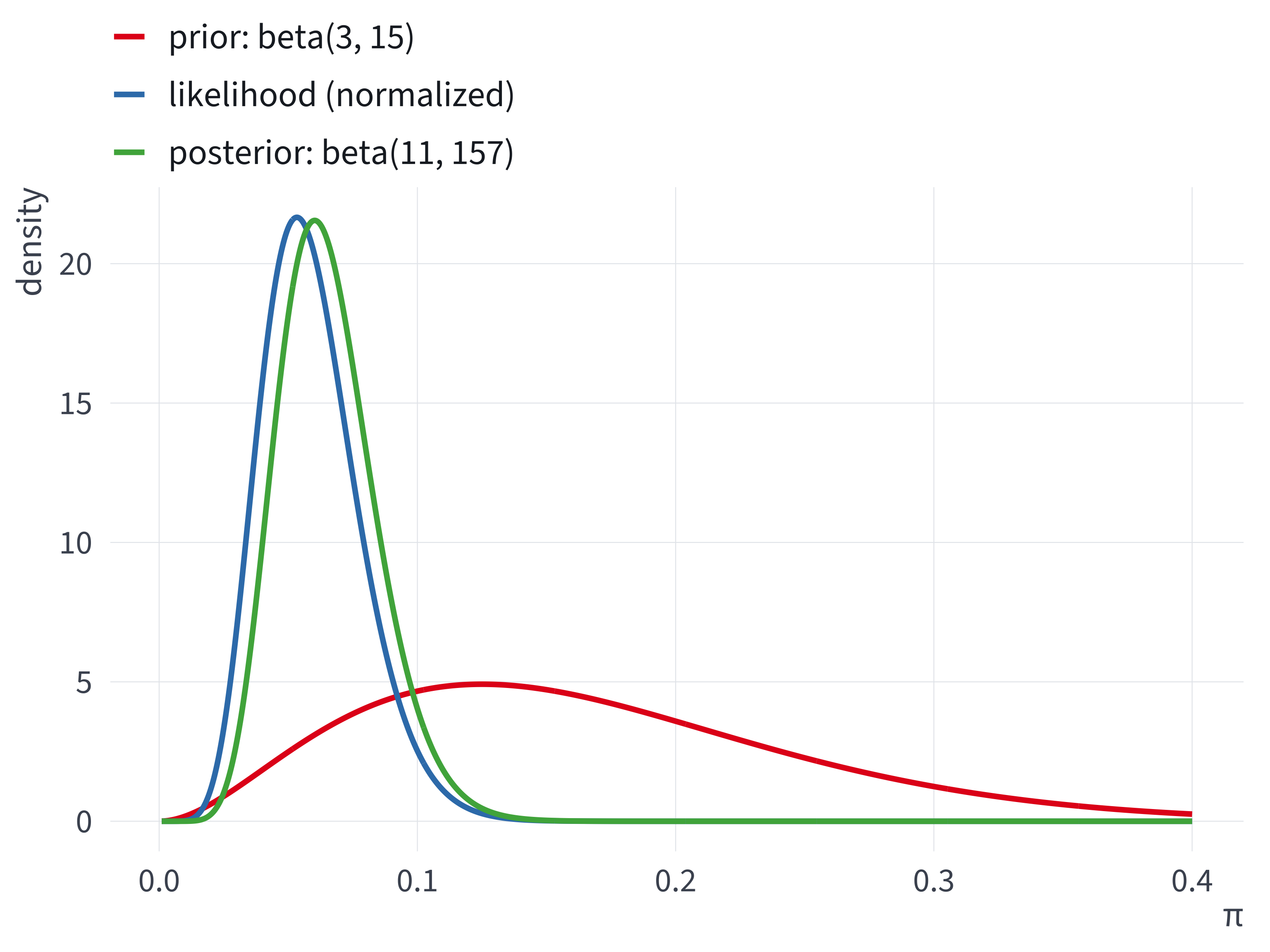
• prior: \(\text{beta}(3, 15)\)
• data: \(k = 8\) tops in \(N = 150\) tosses
• posterior: \(\text{beta}(3 + 8, 15 + 150 - 8)\) \(= \text{beta}(11, 157)\)

Bayes’ rule → posterior → sample

Recap from the Week 6 notes (01-bayes). The likelihood is drawn as a density (beta(9, 143)) so it shares the axis with the prior and posterior. [CTK: the point of the arrow: in most applied cases we can only sample from the posterior.]

Last week: rejection sampling

Algorithm: Rejection Sampling

Inputs:

• The unnormalized posterior \(f(\pi \mid y)\) on \([0, 1]\).
• Desired number of draws \(S\).
• Envelope constant \(M\) such that \(M > f(\pi)\ \forall \pi\).

Algorithm:

1. Initialize: Set \(s = 1\).
2. Repeat while \(s \le S\):
   1. \(z \sim \text{Uniform}(0, 1)\).
   2. \(u \sim \text{Uniform}(0, 1)\).
   3. Accept–reject step: If \(u \leq f(z)/M\), accept: set \(\pi^{(s)} = z\), \(s \leftarrow s + 1\). Otherwise, reject \(z\) and return to Step 2a.

Output: \(\pi^{(1)}, \pi^{(2)}, \ldots, \pi^{(S)} \sim f(\pi \mid y)\).

Footnote from the Keynote box: To make the rejection algorithm simple, I’ve written it to apply specifically to the posterior for the Bernoulli model, which has support [0, 1]. The target density doesn’t need to be a posterior and can have support other than [0, 1]. The proposal distribution doesn’t have to be uniform. The key is that M is larger than the maximum of the target distribution and draws are accepted with probability f(z)/M.

Two costs of rejection

The rejection algorithm is simple and intuitive, but requires

1. finding a suitable envelope constant and
2. rejecting many samples in realistic problems (e.g., logistic regression).

From the opening paragraph of notes/wk07/01-metrop.qmd. [CTK: why both costs get worse in realistic problems, e.g., five coefficients in a logit.]

Rejection sampling for a logit

Let’s use the logit model of the turnout dataset and consider three approaches to sampling from the posterior: rejection (Week 6), Metropolis, and Stan.

The code below applies the simple rejection algorithm we saw for a 1d problem bounded between 0 and 1 to a multidimensional, unbounded problem (i.e., estimating logit coefficients).

# data and design matrix, with rescaled predictors (as in the notes)
turnout <- ZeligData::turnout |>
  mutate(across(age:income, arm::rescale, .names = "rs_{.col}"))
f <- vote ~ rs_age + rs_educate + rs_income + race
X <- model.matrix(f, data = turnout)
y <- turnout$vote

Setup chunk of the exercise “Three samplers, one posterior” (wk07-exercises.qmd), verbatim. The posterior is identical for all three samplers: rescaled predictors with a normal(0, 5) prior on each coefficient, the notes’ logit.stan.

The log posterior and \(M\)

# unnormalized log posterior for many values of beta at once
# - beta has one row per value of beta; the result has one log posterior per row
# - normal(0, 5) prior on each coefficient, same as logit.stan
log_post_many <- function(beta, y, X) {
  eta <- X %*% t(beta)  # one column per row of beta
  log_lik <- colSums(y * eta - (pmax(eta, 0) + log1p(exp(-abs(eta)))))  # stable log(1 + exp(eta))
  log_prior <- rowSums(dnorm(beta, mean = 0, sd = 5, log = TRUE))
  log_lik + log_prior
}

# the same log posterior for a single value of beta
log_post <- function(beta, y, X) {
  log_post_many(matrix(beta, nrow = 1), y, X)
}

# log M: the log posterior at its peak
opt <- optim(rep(0, ncol(X)), log_post, y = y, X = X,
             method = "BFGS", control = list(fnscale = -1))
log_M <- opt$value

[CTK: the envelope constant M is the posterior at its mode, found with optim(); last week M was read off a one-dimensional plot.]

rej_box(): a box from −2 to 2 for every coefficient

The code below creates rej_box(), which works in batches of one million proposals (!!).

rej_box <- function(lower, upper, log_M, y, X, S = 1000, max_batches = 10,
                    batch_size = 1e6, chunk_size = 1e4) {
  start_time <- Sys.time()
  k <- length(lower)
  samples <- matrix(NA_real_, nrow = 0, ncol = k)
  for (b in 1:max_batches) {
    n_accepted_batch <- 0
    # evaluate the batch in chunks (a million proposals at once uses too much memory)
    for (chunk in 1:(batch_size / chunk_size)) {
      # propose: one row per proposal, uniform within the box
      z <- matrix(runif(chunk_size * k, lower, upper), ncol = k, byrow = TRUE)
      # accept with probability f(z) / M
      accept <- log(runif(chunk_size)) <= log_post_many(z, y, X) - log_M
      samples <- rbind(samples, z[accept, , drop = FALSE])
      n_accepted_batch <- n_accepted_batch + sum(accept)
    }
    message("Batch ", b, " of ", max_batches, ": evaluated ",
            scales::comma(batch_size), " proposals... ",
            n_accepted_batch, " accepted (", nrow(samples), " accepted so far; ",
            "worked for ", prettyunits::pretty_dt(Sys.time() - start_time), " so far)")
    if (nrow(samples) >= S) break
  }
  time_total <- Sys.time() - start_time
  message("⏰ Total time: ", prettyunits::pretty_dt(time_total))
  colnames(samples) <- colnames(X)
  list(samples = head(samples, S), n_proposals = b * batch_size,
       time_total = as.numeric(time_total, units = "secs"))
}

Verbatim from the exercise. The highlighted lines are the whole algorithm: propose uniformly inside the box, accept with probability f(z)/M. Everything else is bookkeeping.

Ten million proposals

set.seed(1234)
rej_wide <- rej_box(lower = rep(-2, 5), upper = rep(2, 5),  # the box: -2 to 2 for each of the 5 coefficients
                    log_M = log_M, y = y, X = X,
                    S = 1000,          # stop once 1,000 draws are accepted
                    max_batches = 10,  # ...or after 10 batches, whichever comes first
                    batch_size = 1e6,  # one million proposals per batch (one progress message per batch)
                    chunk_size = 1e4)  # evaluate each batch 10,000 proposals at a time (to save memory)

Batch 1 of 10: evaluated 1,000,000 proposals... 0 accepted (0 accepted so far; worked for 42.2s so far)

Batch 2 of 10: evaluated 1,000,000 proposals... 4 accepted (4 accepted so far; worked for 1m 24.5s so far)

Batch 3 of 10: evaluated 1,000,000 proposals... 0 accepted (4 accepted so far; worked for 2m 6.6s so far)

Batch 4 of 10: evaluated 1,000,000 proposals... 0 accepted (4 accepted so far; worked for 2m 48.5s so far)

Batch 5 of 10: evaluated 1,000,000 proposals... 1 accepted (5 accepted so far; worked for 3m 30.6s so far)

Batch 6 of 10: evaluated 1,000,000 proposals... 2 accepted (7 accepted so far; worked for 4m 12.8s so far)

Batch 7 of 10: evaluated 1,000,000 proposals... 1 accepted (8 accepted so far; worked for 4m 54.4s so far)

Batch 8 of 10: evaluated 1,000,000 proposals... 1 accepted (9 accepted so far; worked for 5m 36.6s so far)

Batch 9 of 10: evaluated 1,000,000 proposals... 1 accepted (10 accepted so far; worked for 6m 18.5s so far)

Batch 10 of 10: evaluated 1,000,000 proposals... 1 accepted (11 accepted so far; worked for 7m 0.2s so far)

⏰ Total time: 7m 0.2s

Ten batches of one million proposals, as in the exercise. The exercise’s hint: the share of proposals accepted estimates the acceptance rate; divide 1,000 by that rate to find the number of proposals you need.

The acceptance rate

# acceptance rate, and what 1,000 draws would take
n_accepted <- nrow(rej_wide$samples)
rate <- n_accepted / rej_wide$n_proposals
proposals_needed <- 1000 / rate
hours_needed <- proposals_needed * (rej_wide$time_total / rej_wide$n_proposals) / 3600
c(accepted = n_accepted, rate = rate,
  proposals_needed = proposals_needed, hours_needed = hours_needed)

        accepted             rate proposals_needed     hours_needed 
        1.10e+01         1.10e-06         9.09e+08         1.06e+01 

We accepted 11 of 10 million proposals in 7 minutes. That’s an acceptance rate of about 1.1 × 10⁻⁶. At that rate, 1,000 draws would take about 910 million proposals (about 11 hours).

The exercise’s rejection part, given away: the solution’s sentence, with this render’s numbers. [CTK: why so few: the posterior occupies a tiny fraction of the five-dimensional box, and f(z)/M is tiny everywhere else. See the next slide.]

The accepted draws

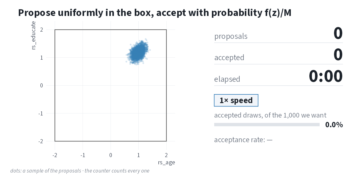
Left: the proposal box, −2 to 2, in two of its five dimensions. Blue: 4,000 draws from the normal approximation to the posterior (glm() coefficients and covariance). Red: the 11 accepted draws. Gray dots: a sample of the proposals. Right: the counters count every proposal. The speed matches the real computation for the first six seconds, then it speeds up.

The run from the previous two slides, as it happened: the hidden chunk after the run replays its random stream to recover when each draw was accepted, checks that the replay matches rej_wide exactly, and rebuilds img/rej-sampler.gif (shown on click; img/rej-sampler-start.png is its first frame, extracted with {magick}) with wk07-lecture-material/rej-gif/make-rej-gif.R from the run’s own count and time, so the draws, the rate, and the hours here are the slide’s numbers. Added 2026-10-06 for the [CTK] cue after “Two costs of rejection”.

[CTK: the accepted draws sit where the posterior is; the box is enormous by comparison, and in five dimensions the ratio of volumes is far smaller than this two-dimensional picture shows. This is cost 2 from two slides ago, made concrete. Metropolis and Stan get the same posterior in seconds; that is Part 1 and Part 2 of the exercise.]

Beyond rejection

We can improve the rejection algorithm by making proposals that depend on the current value.

Notes continue: Many algorithms, including Stan, do this. The Metropolis algorithm is one example.

Metropolis

MCMC

The Metropolis algorithm belongs to a larger class of Markov chain Monte Carlo (MCMC) algorithms, which includes Metropolis-Hastings, Gibbs sampling, and the Hamiltonian Monte Carlo algorithm used by Stan.

MCMC refers to a family of algorithms for generating samples from a target probability distribution by constructing a Markov chain whose stationary distribution is that target. Over many iterations, the samples produced by the chain approximate (dependent) draws from the posterior distribution, allowing us to estimate quantities such as means, variances, and credible intervals even when the posterior cannot be computed analytically.

Metropolis

Algorithm: Metropolis

Inputs:

• The unnormalized log-posterior \(\log f(\theta\mid y)\).
• Desired number of iterations \(S\). Note: the samples are dependent so choose large \(S\) (e.g., \(S = 20{,}000\)), perhaps very large (e.g., \(S = 200{,}000\)).
• Tuning parameter \(\tau\), which controls the width of the uniform proposal density.

Algorithm:

• Initialize: Choose an initial \(\theta^{(1)}\). Set \(s=1\).
• Repeat until \(s=S\):
  • Propose: Draw \(z\) from a uniform distribution from \([\theta^{(s)} - \tau]\) to \([\theta^{(s)} + \tau]\).
  • Compute log-acceptance: \(\Delta = \log f(z)-\log f \big(\theta^{(s)}\big)\)
  • Accept/reject: Draw \(u \sim \text{Uniform}(0,1)\). Accept iff \(\log u \le \Delta\). If accept, set \(\theta^{(s+1)}=z\); otherwise \(\theta^{(s+1)}=\theta^{(s)}\).
  • Iterate: \(s\leftarrow s+1\).

Output: A Markov chain \(\{\theta^{(s)}\}_{s=1}^S\) with stationary distribution \(f(\theta\mid y)\). Consecutive draws are not independent; in practice, discard a burn-in and tune \(\tau\) to maintain a reasonable acceptance rate (perhaps 0.2-0.5, problem-dependent).

Accept/reject

Importantly, this accepts with probability equal to \(\dfrac{f(\text{proposal})}{f(\text{current})}\) if the ratio is between zero and one and always if the ratio is greater than one.

This step is similar to the rejection algorithm, except we keep the current value in place of the rejected proposal in Metropolis.

Both sentences are the footnote to the accept/reject step in the notes. [CTK: contrast with last week: rejection throws the proposal away and tries again; Metropolis writes down the current value again.]

The algorithm, one iteration at a time

The walker animation (wk07-slides-material/figs/fig-metropolis-walker.gif) cut into 43 segments that advance on click: the first plays on arrival, each click plays the next and holds its last frame. 42 clicks in all. Segment ends (iteration-step) and lengths:

1. 1-intro (1.0 s)
2. 2-propose (0.8 s)
3. 2-compute (0.8 s)
4. 2-draw_u (0.5 s)
5. 2-decide (0.8 s)
6. 2-record (0.6 s)
7. 3-propose (0.8 s)
8. 3-compute (0.8 s)
9. 3-draw_u (0.5 s)
10. 3-decide (0.8 s)
11. 3-record (0.6 s)
12. 4-propose (0.5 s)
13. 4-compute (0.5 s)
14. 4-draw_u (0.5 s)
15. 4-decide (0.5 s)
16. 4-record (0.5 s)
17. 5-propose (0.5 s)
18. 5-compute (0.5 s)
19. 5-draw_u (0.5 s)
20. 5-decide (0.5 s)
21. 5-record (0.5 s)
22. 18-zoom (13.8 s)
23. 19-propose (0.8 s)
24. 19-compute (0.8 s)
25. 19-draw_u (0.8 s)
26. 19-decide (0.8 s)
27. 19-record (0.6 s)
28. 20-propose (0.8 s)
29. 20-compute (0.8 s)
30. 20-draw_u (0.8 s)
31. 20-decide (0.8 s)
32. 20-record (0.6 s)
33. 21-propose (0.8 s)
34. 21-compute (0.8 s)
35. 21-draw_u (0.8 s)
36. 21-decide (0.8 s)
37. 21-record (0.6 s)
38. 22-propose (0.6 s)
39. 22-compute (0.6 s)
40. 22-draw_u (0.8 s)
41. 22-decide (0.8 s)
42. 22-record (0.6 s)
43. 36-hold (16.0 s)

A clicker’s next button sends Right or Page Down, which reveal maps to the next fragment, so nothing needs configuring. Clicking while a segment is still playing skips to the next one; Left steps back to the previous segment’s last frame.

[CTK: the pause points are the stops table at the top of make-walker-segments.R; edit it and re-run the script to reshape the clicks.]

metrop()

metrop <- function(logf, theta_start, S = 10000, tau = 0.1, ...) {
  # initialize matrix of samples with starting values
  k <- length(theta_start)
  samples <- matrix(NA_real_, nrow = S, ncol = k)
  samples[1, ] <- theta_start

  # proceed with algorithm
  for (s in 2:S) {
    # extract current location
    current <- samples[s - 1, ]

    # generate symmetric random-walk proposal
    proposed_move <- runif(k, -tau, tau)
    proposal <- current + proposed_move

    # acceptance step
    delta <- logf(proposal, ...) - logf(current, ...)
    if (delta > 0) {
      accept <- TRUE
    } else {
      accept <- (log(runif(1)) <= delta)
    }

    # update samples
    if (accept) {
      samples[s, ] <- proposal
    } else {
      samples[s, ] <- current
    }
  }

  # return a list, so the samples are m$samples
  list(samples = samples)
}

This is the minimal version from the notes, except that it returns list(samples = samples) rather than the bare matrix, so m$samples works on every later slide. The in-class scripts (wk07-toothpaste-metropolis.R, wk07-logit-metropolis.R) use the “some features added” version: same algorithm, plus a progress bar, the acceptance rate, and a reminder message. It returns a list, so the code from here on uses m$samples. The deck runs that version too (hidden chunk).

Toothpaste cap

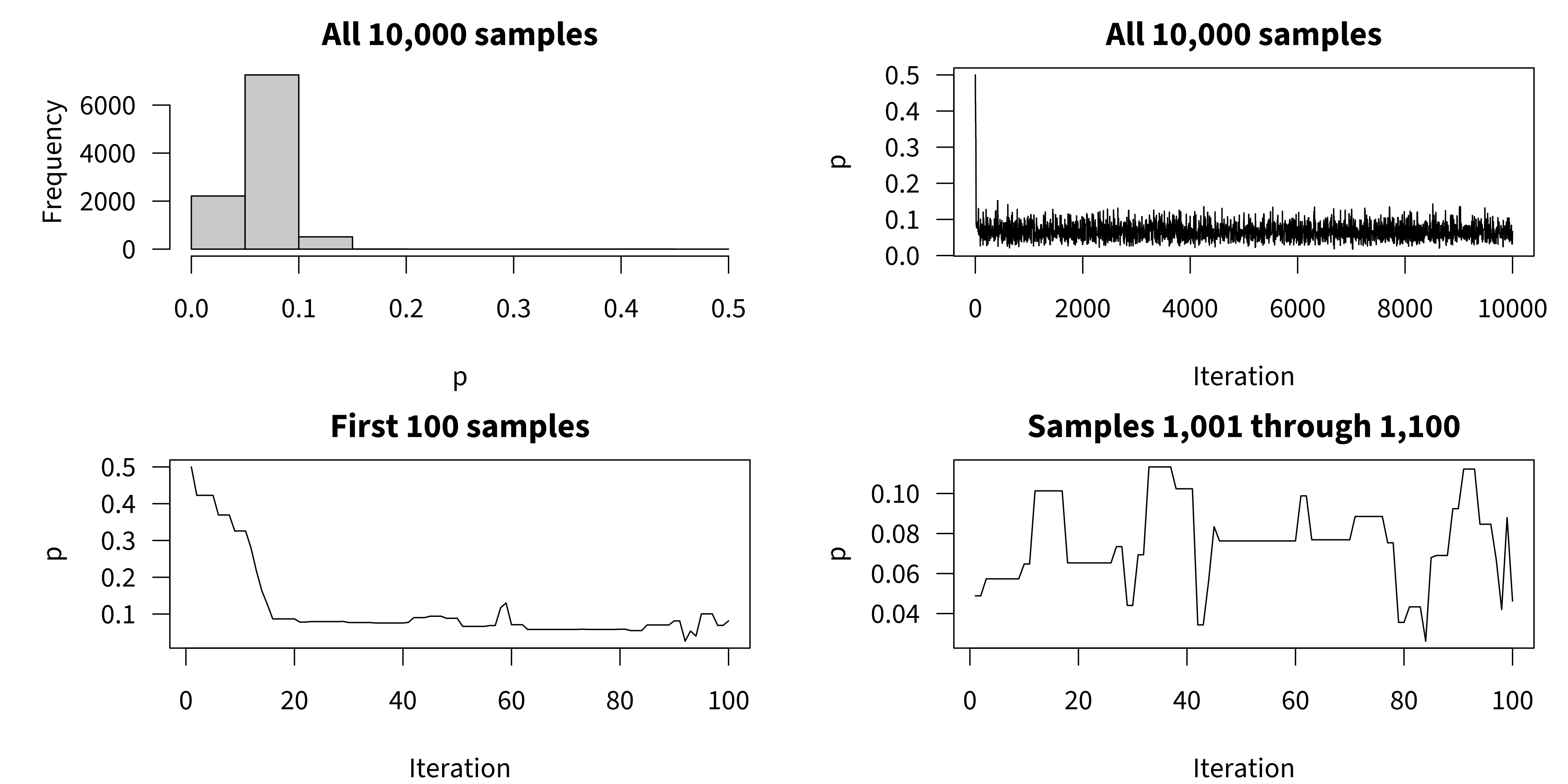
For \(k=8\) and \(N=150\) with a \(\text{beta}(3, 15)\) prior, the posterior is \(\text{beta}(11,157)\).

# create log-target for Beta posterior; -Inf outside (0,1)
logf <- function(p) {
  ifelse(p <= 0 | p >= 1,
         -Inf,
         dbeta(p, 11, 157, log = TRUE))
}

# run algorithm starting in the middle of (0,1)
set.seed(1234)
m <- metrop(
  logf,            # log-target
  theta_start = 0.5
)

# closed-form posterior mean
11 / (11 + 157)

[1] 0.0655

# simulations (samples is S x k; here k = 1)
mean(m$samples)

[1] 0.0662

Toothpaste cap: the samples

Two things worth noting

1. The samples are not independent. Many consecutive draws are identical (rejections) or move only a little; the chain explores the target slowly.
2. It takes a few iterations for the chain to reach the high-probability region (burn-in). Starting at \(\pi=0.5\) is far from the posterior mass; it takes roughly a few dozen iterations to reach \(\approx 0.1\).

Burn-in

The MCMC samples are heavily dependent on the starting values, so discard early samples that depend strongly on the starting value (the “burn-in”). Discarding the first 10% to 50% of the samples is typical.

# simulations, keep only samples 5,001 through 10,000 (discard first half)
mean(m$samples[5001:10000, 1])

[1] 0.0652

Aside from the notes: Stan and {brms} call this period the “warmup” rather than the burn-in. During warmup, Stan’s sampler also tunes itself (e.g., its step size), so the warmup samples are not draws from a fixed algorithm. Our Metropolis sampler keeps tau fixed, so “burn-in” fits here.

R-hat

But how do we know how long to run our algorithms? How do we know if the samples have converged to the target distribution? This is still a difficult problem.

No diagnostic can show that the chains have converged, but R-hat can show that they have not. We check that R-hat is less than 1.01 (Vehtari et al. 2021).

To compute R-hat, run several chains from overdispersed starting values. It is important that these be high and low relative to the target distribution. If chains have converged, within- and between-chain variation align and \(\hat{R}\approx 1\).

Notes continue: If R-hat is larger than 1.01, the chains have not converged and we need more iterations. If R-hat is less than 1.01, we have found no sign of a problem. Aside from the notes: {brms} warns only when some R-hat is larger than 1.05. We use the stricter threshold of 1.01 from Vehtari et al. (2021), so check R-hat yourself even when {brms} prints no warning.

R-hat: 25 iterations

# run algorithm four times, making four "chains"
set.seed(1234)
m1 <- metrop(logf, theta_start = 0.01, S = 25)
m2 <- metrop(logf, theta_start = 0.25, S = 25)
m3 <- metrop(logf, theta_start = 0.75, S = 25)
m4 <- metrop(logf, theta_start = 0.99, S = 25)

# a matrix of chains for first (and only) dimension
matrix_of_chains <- cbind(
  m1$samples[, 1],
  m2$samples[, 1],
  m3$samples[, 1],
  m4$samples[, 1]
)

# compute r-hat using the rhat() function in {posterior}
posterior::rhat(matrix_of_chains)

[1] 2.43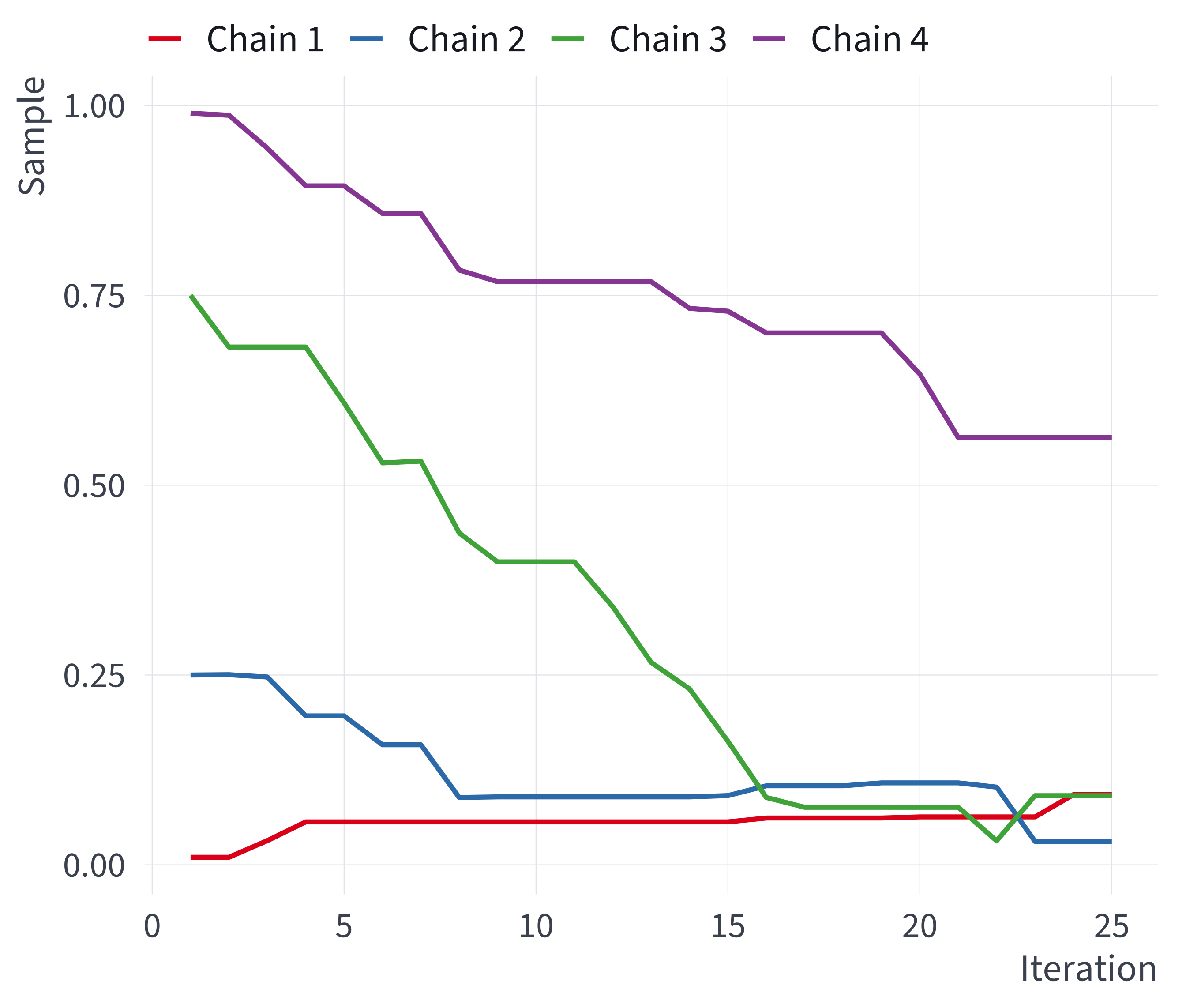

R-hat: 25,000 iterations, first 10,000 discarded

# run algorithm four times, making four "chains"
set.seed(1234)
m1 <- metrop(logf, theta_start = 0.01, S = 25000)
m2 <- metrop(logf, theta_start = 0.25, S = 25000)
m3 <- metrop(logf, theta_start = 0.75, S = 25000)
m4 <- metrop(logf, theta_start = 0.99, S = 25000)

# a matrix of chains for first (and only) dimension
matrix_of_chains <- cbind(
  m1$samples[10001:25000, 1],
  m2$samples[10001:25000, 1],
  m3$samples[10001:25000, 1],
  m4$samples[10001:25000, 1]
)

# compute r-hat using the rhat() function in {posterior}
posterior::rhat(matrix_of_chains)

[1] 1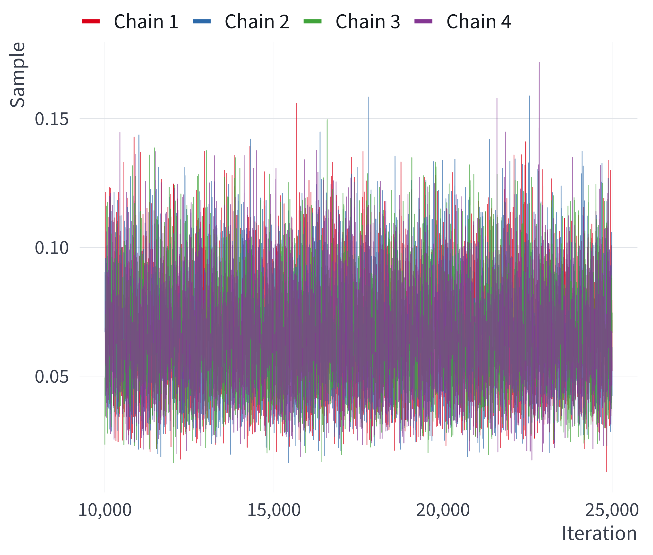

If we increase S to a larger value and discard the initial samples, then R-hat falls below 1.01.

Parallel chains

# overdispersed starting values
starting_values <- seq(0.05, 0.95, length.out = 10)

# one core per chain, but no more than the machine has
n_cores <- min(10, parallel::detectCores(logical = FALSE))
cl <- makeCluster(n_cores)
clusterSetRNGStream(cl, iseed = 1234)  # reproducible draws on the workers
registerDoParallel(cl)

# run 10 chains in parallel; combine samples with cbind()
matrix_of_chains <- foreach(s = starting_values,
                            .combine = cbind) %dopar% {
  m <- metrop(logf, theta_start = s, S = 25)
  m$samples
}
stopCluster(cl)

# compute R-hat using {posterior}
posterior::rhat(matrix_of_chains)

[1] 2.3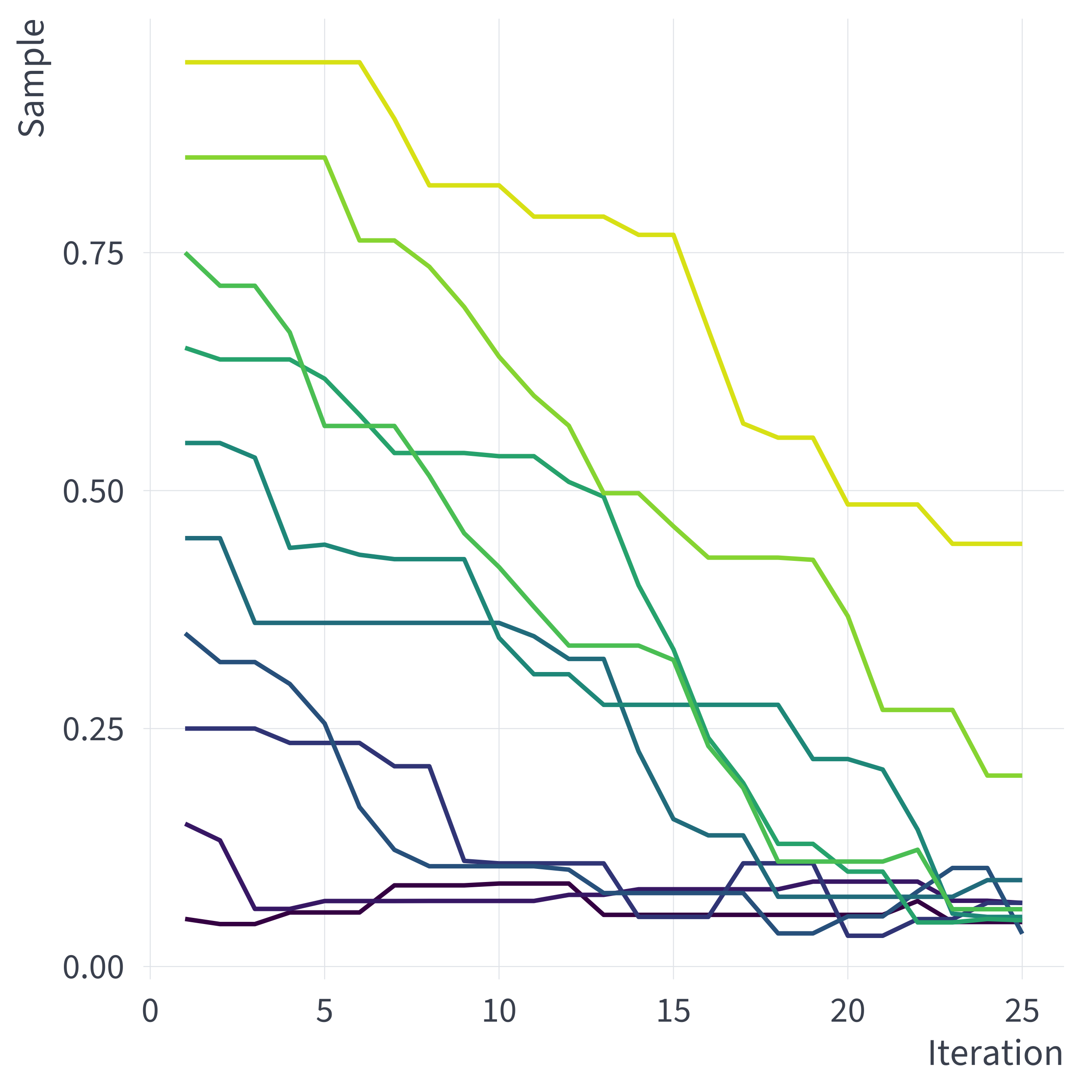

Notes: Multiple chains are naturally parallelizable. In fact, these are called “embarrassingly parallel,” because the chains are run entirely independently. Nothing from the first chain is needed for the second, and so on. The figure shows the 25 samples from each of the 10 chains. Notice the strong dependence on starting values! In practice, we’d need to generate many more samples, discard the first samples, and check that R-hat is less than 1.01. The in-class script uses S = 250 here; the notes and this slide use S = 25.

ESS

Dependent Metropolis samples carry less information than the same number of independent samples.

Effective Sample Size (ESS): “our dependent samples are like ______ independent samples.”

# the four long chains from above, minus the first 10,000 samples of each
matrix_of_chains <- cbind(
  m1$samples[10001:25000, 1],
  m2$samples[10001:25000, 1],
  m3$samples[10001:25000, 1],
  m4$samples[10001:25000, 1]
)
dim(matrix_of_chains)  # 15,000 x 4 = 60,000 samples

[1] 15000     4

# are like
posterior::ess_bulk(matrix_of_chains)  # ESS for the center of the distribution

[1] 11909

posterior::ess_tail(matrix_of_chains)  # ESS for tail estimands

[1] 12715

Notes: The Effective Sample Size (ESS) summarizes the amount of information in our dependent samples. The literature and practices on ESS are evolving rapidly; see ?posterior::ess_bulk for the latest references.

Tuning \(\tau\)

# varying the tuning parameter tau
set.seed(1234)
m1 <- metrop(logf, theta_start = 0.99, S = 1000, tau = 0.1)
m2 <- metrop(logf, theta_start = 0.99, S = 1000, tau = 0.01)
m3 <- metrop(logf, theta_start = 0.99, S = 1000, tau = 0.001)
m4 <- metrop(logf, theta_start = 0.99, S = 1000, tau = 3)

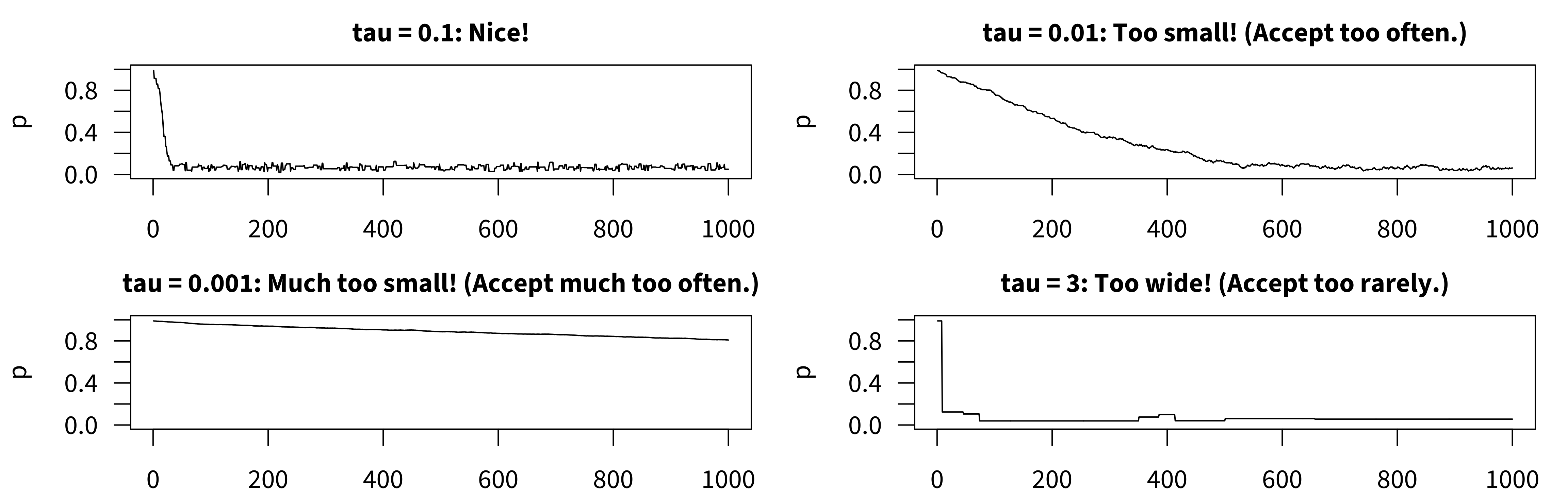
the value of tau should be something like the SD of the posterior

“Something like” means within an order of magnitude. For the toothpaste cap problem, about 5 SDs (tau = 0.1) is about right.

Notes: The tuning parameter matters a lot. I’ve chosen a smart default for many problems, but the value of tau should be something like the SD of the posterior. Measured 2026-10-06 (grid of tau, 20,000 draws, ESS per draw): the posterior SD of beta(11, 157) is 0.019; efficiency peaks near tau = 4 SD (acceptance about 40%), and tau = 0.1 (5.3 SD) is within about 10% of the peak; tau = SD gives one fifth the effective sample; tau = 3 is wider than the whole support. Theory (Roberts, Gelman & Gilks 1997): optimal proposal SD is about 2.4 posterior SDs in 1-d, shrinking as 1/sqrt(d); a uniform on +/- tau has SD tau/sqrt(3), so the optimal half-width is about 4 SD in 1-d and about 1.8 SD for the 5-parameter logit (measured optimum 1.5-2 SD, acceptance about 20%).

Why the Metropolis algorithm works

Symmetric proposals give equal opportunity.

• From any point \(x\), the chance of proposing \(z\) is the same as proposing \(x\) from \(z\).
• The proposal distribution itself doesn’t favor any direction.

Asymmetric acceptance adds the right bias.

• Moves to higher density are always accepted.
• Moves to lower density are accepted with probability \(f(z)/f(x)\).
• This rule makes the chain linger in high-density regions.

Why the Metropolis algorithm works

Balanced flows keep the target intact.

• Although proposals are symmetric, the acceptance rule ensures that the expected number of transitions \(A \rightarrow B\) equals those from \(B \rightarrow A\).
  • From higher-density \(A\) to lower-density \(B\): the chain is at \(A\) often (every proposal toward \(A\) is accepted, so it is easy to get there), but it leaves \(A\) for \(B\) only sometimes, with probability \(f(B)/f(A)\).
  • From lower-density \(B\) to higher-density \(A\): the chain is at \(B\) less often (proposals toward \(B\) are often rejected), but whenever it is at \(B\) and proposes \(A\), it always moves.
  • Many visits times a fraction of exits equals few visits times certain exits: \(f(A) \cdot \frac{f(B)}{f(A)} = f(B) \cdot 1\). The two flows match.
• This condition guarantees that the samples are stationary.

Long-run behavior reflects probability mass.

• Because the chain moves through the space according to these balanced transition rules, it spends time in each region in proportion to its probability under the target.
• In the long run, the sample frequencies mirror the target distribution.

A weird posterior

# sawtooth log-prior (unnormalized):
# log of ((n_teeth*p) %% 1) on (0,1)
log_prior_saw <- function(p, n_teeth = 5) {
  ifelse(p <= 0 | p >= 1, -Inf, log((n_teeth * p) %% 1))
}

# likelihood for 10 tosses w/ one success
log_lik <- function(p) {
  ifelse(p <= 0 | p >= 1, -Inf,
         dbinom(1, size = 10, prob = p, log = TRUE))
}

# log-posterior
log_post <- function(p) log_lik(p) + log_prior_saw(p)

# run metropolis algorithm
set.seed(1234)
m <- metrop(log_post, theta_start = 0.5)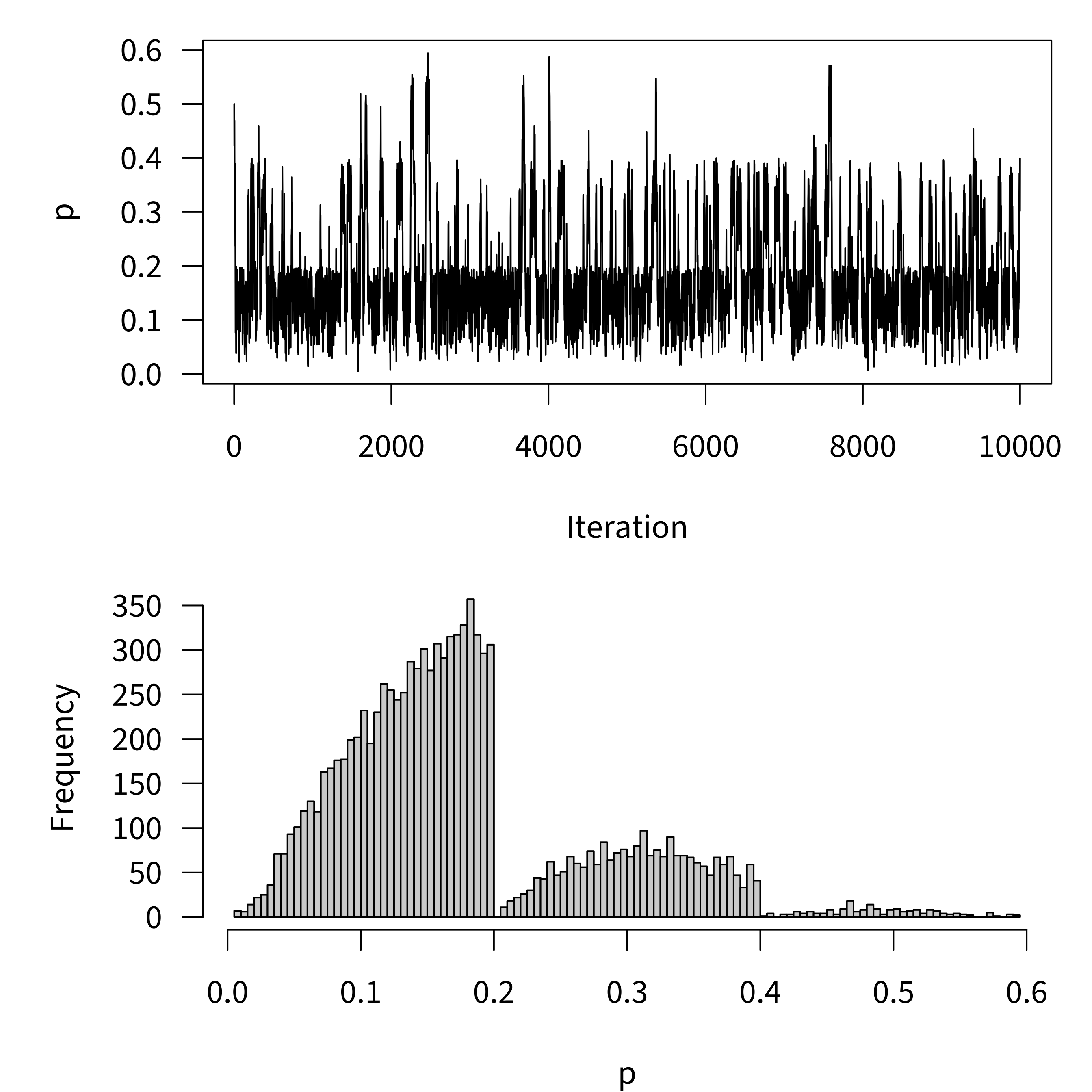

Notes: We can use the Metropolis algorithm for our “weird” sawtooth posterior. We’ll use the log-posterior in this case.

Logistic regression: data

# load only the turnout data frame
turnout <- ZeligData::turnout

# alias for arm::rescale(): mean 0, SD 0.5
rs <- function(x) { arm::rescale(x) }

# create the rescaled variables as columns
turnout <- turnout |>
  mutate(across(age:income, rs, .names = "rs_{.col}"))
f <- vote ~ rs_age + rs_educate + rs_income + race

# fit logit model
fit <- glm(f, family = binomial, data = turnout)

# print estimates
arm::display(fit, digits = 4)

glm(formula = f, family = binomial, data = turnout)
            coef.est coef.se
(Intercept) 1.0578   0.1396 
rs_age      0.9934   0.1212 
rs_educate  1.1837   0.1370 
rs_income   1.0013   0.1535 
racewhite   0.2508   0.1465 
---
  n = 2000, k = 5
  residual deviance = 2024.0, null deviance = 2266.7 (difference = 242.8)

Notes: Recall the logit model from a previous chapter. This time, let’s rescale the numeric variables to have mean of zero and SD of 0.5. This keeps coefficients on a similar scale, which helps us with the computation. For more on this rescaling strategy and its advantages, see Gelman (2008). Code comment in the notes: rescaling inside the formula (e.g., rs(age)) breaks predictions on new data, because rescale() would then use the new data’s mean and SD.

Log-posterior: unstable

For this example, we imagine an improper, constant prior.

# make X and y
mf <- model.frame(f, data = turnout)
X <- model.matrix(f, data = mf)
y <- model.response(mf)

# ❌ correct, but unstable, log unnormalized posterior (flat prior, so just the log-likelihood)
log_posterior <- function(beta, y, X) {
  linpred <- X %*% beta
  # for large |linpred|, plogis() rounds to exactly 0 or 1, so dbinom() returns -Inf;
  #   if the current and proposed values are both -Inf, delta = -Inf - (-Inf) = NaN
  sum(dbinom(y, size = 1, prob = plogis(linpred), log = TRUE))
}

Log-posterior: stable

Why the previous version is unstable. plogis(linpred) rounds to exactly 1 when linpred > 37 and to exactly 0 when linpred < −745. For an observation on the wrong side, dbinom(..., log = TRUE) returns log(0) = −Inf, so the whole sum is −Inf. A −Inf proposal is harmless (rejected), but if the current value is also −Inf (a wild start), delta = −Inf − (−Inf) = NaN and if (delta > 0) errors.

The fix: never compute the probability. Since \(\log \pi = \eta - \log(1 + e^\eta)\) and \(\log(1 - \pi) = -\log(1 + e^\eta)\), the log-likelihood is \(\sum_i [y_i \eta_i - \log(1 + e^{\eta_i})]\). Compute \(\log(1 + e^\eta)\) so that exp() never overflows and log1p() keeps precision when its argument is tiny.

# ✅ same unnormalized log posterior, but computed on the log scale to avoid rounding
log_posterior <- function(beta, y, X) {
  linpred <- drop(X %*% beta)                        # eta; drop() makes it a vector
  log1pexp <- ifelse(linpred > 0,
                     linpred + log1p(exp(-linpred)),  # eta > 0: exp(-eta) <= 1, cannot overflow
                     log1p(exp(linpred)))             # eta <= 0: exp(eta) <= 1; log1p() exact for tiny x
  sum(y * linpred - log1pexp)                        # = sum(y*log(pi) + (1 - y)*log(1 - pi)), finite for every eta
}

At \(\beta = (40, 0, 0, 0, 0)\), the unstable version returns −Inf; this one returns −20,320.

Checked 2026-10-06: from the deck’s four starting values (−2, −1, 1, 2) the unstable version never hits the rounding, so both versions give identical chains here; from a start of 40 the unstable chain errors on its first step (“missing value where TRUE/FALSE needed”) and the stable one runs. The two versions agree to 2e-5 at eta = 20. The notes chapter’s comment on the unstable version says “0*Inf”; the mechanism is log(0) = -Inf (dbinom with prob exactly 0 or 1), then -Inf - (-Inf) = NaN in the acceptance step.

Running the algorithm

# sample with metropolis
set.seed(1234)
S <- 20000
m1 <- metrop(log_posterior, S = S, tau = 0.1,
             theta_start = rep(-2, ncol(X)), y = y, X = X)
m2 <- metrop(log_posterior, S = S, tau = 0.1,
             theta_start = rep(-1, ncol(X)), y = y, X = X)
m3 <- metrop(log_posterior, S = S, tau = 0.1,
             theta_start = rep(1, ncol(X)), y = y, X = X)
m4 <- metrop(log_posterior, S = S, tau = 0.1,
             theta_start = rep(2, ncol(X)), y = y, X = X)

Same seed, S, tau, and starting values as wk07-logit-metropolis.R, so the numbers on the next slides match what students get (the script adds progress_bar = TRUE, which does not change the draws).

R-hat and ESS: intercept

# first parameter (intercept); discard the first 20% of each chain as burn-in
start <- .2*S + 1
end <-   S
matrix_of_chains <- cbind(
  m1$samples[start:end, 1],
  m2$samples[start:end, 1],
  m3$samples[start:end, 1],
  m4$samples[start:end, 1]
)

# compute r-hat (for intercept)
posterior::rhat(matrix_of_chains)

[1] 1

# compute ess (for intercept)
posterior::ess_bulk(matrix_of_chains)

[1] 833

posterior::ess_tail(matrix_of_chains)

[1] 1643

Notes: R-hat less than about 1.01; ESS more than about 2,000. [CTK: at S = 20,000 the bulk ESS for the intercept is below the notes’ 2,000 heuristic (see the output); say whether that is enough here or whether students should run longer, as the notes’ 100,000-iteration version does.]

Intercept: four chains

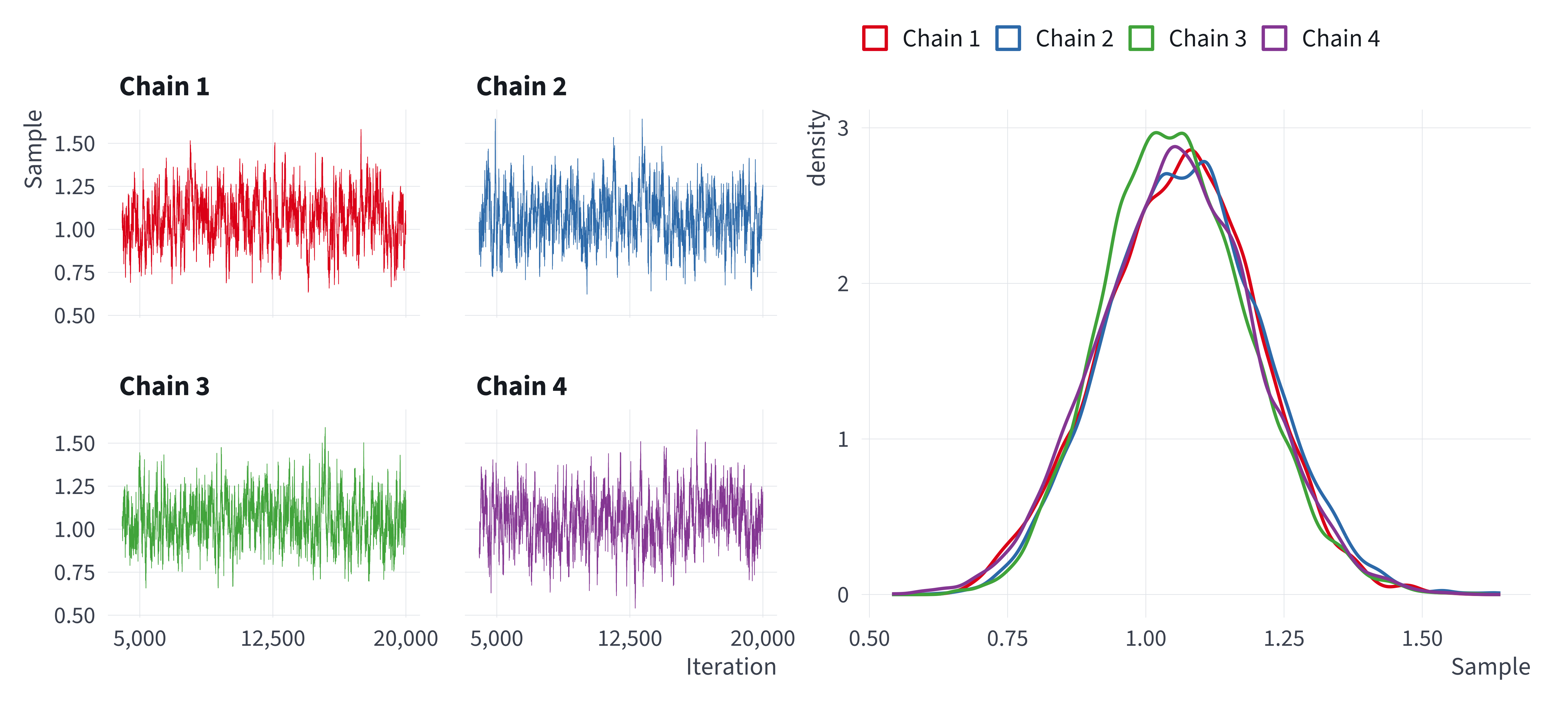
All parameters

Coefficient	R-hat	R-hat < 1.01	ESS (bulk)	ESS (tail)
(Intercept)	1.002	✅	833	1,643
rs_age	1.003	✅	1,176	2,649
rs_educate	1.003	✅	1,092	2,435
rs_income	1.005	✅	914	1,921
racewhite	1.001	✅	864	1,570

Notes: The code above computes the R-hat and ESS for only the first parameter (intercept); we should check the rest as well. Notes: The table below shows that R-hat is less than 1.01 for every parameter, so we have found no sign that the chains have failed to converge. (True at S = 20,000 too; check the rendered column.)

glm() vs. metrop(): point estimates and 95% CIs

Notes: Finally, we can compare the posterior mean and 95% credible intervals to the ML estimate and 95% Wald confidence intervals. They are almost identical. (The notes’ plotting code uses the posterior median for the point; so does this figure.)

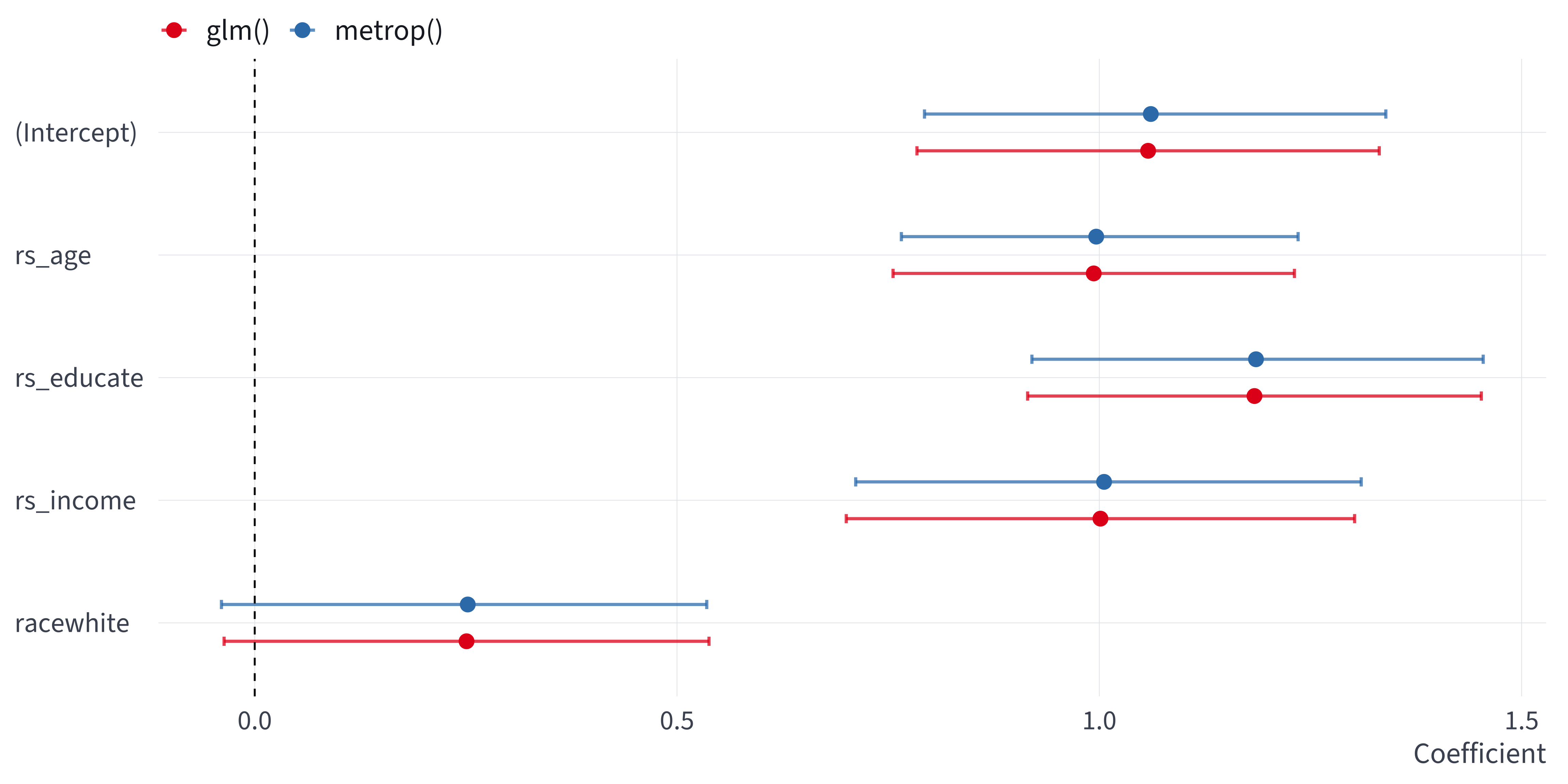
Quantities of interest

To compute a quantity of interest, we need to use our Bayesian invariance property. We need to transform, then summarize, the simulations.

# make X_lo
X_lo <- cbind(
  "constant" = 1, # intercept
  "rs_age" = -0.5, # 1 SD below avg -- see ?arm::rescale
  "rs_educate" = 0,
  "rs_income" = 0,
  "white" = 1 # white indicator = 1
)

# make X_hi by modifying the relevant value of X_lo
X_hi <- X_lo
X_hi[, "rs_age"] <- 0.5  # 1 SD above avg

# function to compute first difference
fd_fn <- function(beta, hi, lo) {
  plogis(hi%*%beta) - plogis(lo%*%beta)
}

Transform, then summarize

# each row is one beta-tilde; discard burn-in; stack the chains
beta_tilde <- rbind(
  m1$samples[start:end, ], # chain 1, minus burn-in
  m2$samples[start:end, ], # chain 2, minus burn-in
  m3$samples[start:end, ], # chain 3, minus burn-in
  m4$samples[start:end, ]  # chain 4, minus burn-in
)

# transform simulations of coefficients into simulations of first-difference
fd_tilde <- numeric(nrow(beta_tilde))  # container
for (i in 1:nrow(beta_tilde)) {
  fd_tilde[i] <- fd_fn(beta_tilde[i, ], hi = X_hi, lo = X_lo)
}

# summarize: posterior mean, posterior SD, and 95% credible interval
mean(fd_tilde)

[1] 0.166

sd(fd_tilde)

[1] 0.0197

quantile(fd_tilde, probs = c(0.025, 0.975))

 2.5% 97.5% 
0.129 0.205 

With {marginaleffects}

# compute qi with the rescaled columns
cmp <- comparisons(fit, variables = list(rs_age = c(-0.5, 0.5)),
                   newdata = datagrid(grid_type = "mean_or_mode"))

# ML estimate, delta-method SE, and 95% confidence interval
cmp |>
  as.data.frame() |>
  select(term, contrast, estimate, std.error, conf.low, conf.high)

    term   contrast estimate std.error conf.low conf.high
1 rs_age 0.5 - -0.5    0.166      0.02    0.127     0.205

[CTK: the two estimates agree; {marginaleffects} gives the ML point estimate with a delta-method interval, metrop() gives the posterior mean of the first difference.]

metrop() vs. comparisons(): the first difference

Method	Estimate	SE	2.5%	97.5%
metrop(): posterior mean, posterior SD, and 2.5th and 97.5th percentiles of the simulated first differences. comparisons(): ML estimate, delta-method standard error, and Wald 95% confidence interval.
metrop(): posterior simulations	0.166	0.020	0.129	0.205
glm() + comparisons(): ML + delta method	0.166	0.020	0.127	0.205

The first difference in Pr(vote) for a 1 SD shift in age (rs_age from -0.5 to 0.5), with education and income at their means and race = white. Same quantity, two routes: the posterior mean and credible interval from the four Metropolis chains stacked, and the ML point estimate with a delta-method interval from comparisons(). They agree to the second decimal.

Summary

MCMC

MCMC offers a powerful and general way to sample from an unnormalized (log-)posterior. The Metropolis algorithm is one such method. Hamiltonian Monte Carlo (HMC) via Stan is even better.

R-hat and burn-in

The first MCMC samples are highly dependent on the starting values. Because of this, you need to:

1. Discard the samples from a burn-in period.
2. Run multiple chains and check that R-hat is less than 1.01.

ESS and large samples

The MCMC samples are dependent on the previous samples. Because of this, you need to:

1. Generate more samples than you would need if they were independent.
2. Use ESS to understand your effective sample size.

Stan

Stan

• Stan offers an extremely efficient alternative to Metropolis and other MCMC algorithms.
• It uses a hyper-optimized version of Hamiltonian Monte Carlo.
• Stan and its universe of supporting software is extremely well-documented and widely used.

• Build note: Keynote “Stan” slide (Fall 2025), two typos fixed.
• From the notes’ aside: Before Stan, Bayesian modeling in R was typically done using BUGS or JAGS, which relied on Gibbs sampling and Metropolis-within-Gibbs updates. Stan uses gradients of the log-posterior to navigate the parameter space more efficiently.
• In-class script: https://pos5747.github.io/files/wk07-logit-stan.R

Logistic regression model

\[ y_i \sim \text{Bernoulli}(\pi_i), \quad \pi_i = \operatorname{logit}^{-1} \left( X_i \beta \right). \]

We’ll assume weakly informative priors (i.e., variance = 25).

\[ \beta \sim \mathcal{N}(0, 5^2 I). \]

Because the scale of the variables affects the interpretation of the priors, it’s common to rescale variables to have a common scale (e.g., SD of 0.5, SD of 1, or range of 1).

• [CTK: the income example from the notes: a prior with an SD of 5 is more or less informative depending on whether income is dollars or thousands of dollars.]

Three blocks

Each Stan model has three main blocks.

1. data { ... } Known inputs provided from R.
2. parameters { ... } Unknowns to infer (e.g., vector[K] beta;, real<lower=0> sigma;). Put constraints that reflect the parameter’s support.
3. model { ... } Priors and likelihood live here. Use distribution statements (theta ~ normal(0,1);)

There are other blocks you can use as well.

• From the notes’ footnote: Stan is a declarative modeling language: you describe the data you have, the parameters you don’t know, and the probabilistic relationships (priors and likelihood) that connect them.
• Documentation: user’s guide, reference manual, tutorials, case studies at https://mc-stan.org.

logit.stan

The Stan model mirrors the math closely.

// data block
data {
  int<lower=0> N;  // rows in design matrix
  int<lower=1> K;  // columns in design matrix
  array[N] int<lower=0, upper=1> y;  // binary outcome
  matrix[N, K] X;  // design matrix
}

// parameters block
parameters {
  vector[K] beta;  // logit coefficients
}

// model block
model {
  beta ~ normal(0, 5);               // n(0, 5) prior for each beta
  y ~ bernoulli_logit(X * beta);     // logistic regression likelihood
}

• Build note: the code highlight steps through the three blocks: data, parameters, model.
• We should save this text file as logit.stan in our project directory.

Data for Stan

# load only the turnout data frame
turnout <- ZeligData::turnout  |>
  # create rescaled columns (rescaling inside the formula breaks predictions on new data)
  mutate(across(age:income, arm::rescale, .names = "rs_{.col}")) |>
  glimpse()

Rows: 2,000
Columns: 8
$ race       <fct> white, white, white, white, white, white, white, white, white, white,…
$ age        <int> 60, 51, 24, 38, 25, 67, 40, 56, 32, 75, 46, 52, 22, 60, 24, 30, 46, 6…
$ educate    <dbl> 14, 10, 12, 8, 12, 12, 12, 10, 12, 16, 15, 12, 12, 12, 14, 10, 12, 9,…
$ income     <dbl> 3.346, 1.856, 0.630, 3.418, 2.785, 2.387, 4.286, 9.320, 3.880, 2.703,…
$ vote       <int> 1, 0, 0, 1, 1, 1, 0, 1, 1, 1, 1, 1, 0, 0, 1, 1, 1, 1, 1, 1, 1, 1, 1, …
$ rs_age     <dbl> 0.4197, 0.1628, -0.6079, -0.2082, -0.5793, 0.6195, -0.1512, 0.3055, -…
$ rs_educate <dbl> 0.2868, -0.3067, -0.0099, -0.6034, -0.0099, -0.0099, -0.0099, -0.3067…
$ rs_income  <dbl> -0.09566, -0.35915, -0.57595, -0.08284, -0.19482, -0.26532, 0.07058, …

Data for Stan

# build model frame
f <- vote ~ rs_age + rs_educate + rs_income + race
mf <- model.frame(f, data = turnout)
X  <- model.matrix(f, data = mf)
y  <- model.response(mf)

# bundle data for Stan
stan_data <- list(
  N = nrow(X),
  K = ncol(X),
  y = as.integer(y),
  X = X
)

Writing logit.stan from R

stan_code <- "
data {
  int<lower=0> N;
  int<lower=1> K;
  array[N] int<lower=0, upper=1> y;
  matrix[N, K] X;
}
parameters {
  vector[K] beta;
}
model {
  beta ~ normal(0, 5);               // weakly informative prior
  y ~ bernoulli_logit(X * beta);     // logistic regression likelihood
}
"
# Write the Stan program so the document runs without external files.
writeLines(stan_code, con = 'logit.stan')

Install {cmdstanr} and CmdStan

{cmdstanr} is not on CRAN, so we install it from the Stan r-universe and then use it to install CmdStan.

install.packages("cmdstanr",
                 repos = c("https://stan-dev.r-universe.dev", getOption("repos")))
cmdstanr::check_cmdstan_toolchain(fix = TRUE)
cmdstanr::install_cmdstan()

• From the notes’ aside: {cmdstanr} is faster and will experience fewer crashes than {rstan}; on Carlisle’s laptop the turnout example takes about 7 seconds in {cmdstanr} and about 24 seconds in {rstan}, almost all of it compile time.

{cmdstanr}

First, we compile the model with cmdstan_model(). Then we draw samples with the $sample() method.

mod <- cmdstan_model("logit.stan")

fit_cmd <- mod$sample(
  data = stan_data,
  chains = 4,
  parallel_chains = 4,  # run the chains in parallel
  iter_warmup = 1000,
  iter_sampling = 2000,  # excluding warmup
  seed = 123
)

$summary()

The $summary() method reports posterior summaries along with R-hat, bulk ESS, and tail ESS for each parameter.

fit_cmd$summary(variables = "beta")

# A tibble: 5 × 10
  variable  mean median    sd   mad      q5   q95  rhat ess_bulk ess_tail
  <chr>    <dbl>  <dbl> <dbl> <dbl>   <dbl> <dbl> <dbl>    <dbl>    <dbl>
1 beta[1]  1.07   1.07  0.141 0.141 0.838   1.30   1.00    4580.    4749.
2 beta[2]  0.994  0.992 0.122 0.121 0.796   1.20   1.00    6150.    5310.
3 beta[3]  1.19   1.19  0.137 0.136 0.963   1.41   1.00    5512.    4635.
4 beta[4]  1.01   1.01  0.153 0.150 0.755   1.26   1.00    6170.    4874.
5 beta[5]  0.246  0.245 0.148 0.149 0.00498 0.490  1.00    4766.    5011.

Diagnostics

• \(\hat{R}\): an R-hat larger than 1.01 shows that the chains have not converged.
• Effective Sample Size (ESS): how much independent information is in the draws.

draws_beta <- fit_cmd$draws(variables = "beta")  # draws array
summarise_draws(draws_beta, "rhat", "ess_bulk", "ess_tail")

# A tibble: 5 × 4
  variable  rhat ess_bulk ess_tail
  <chr>    <dbl>    <dbl>    <dbl>
1 beta[1]   1.00    4580.    4749.
2 beta[2]   1.00    6150.    5310.
3 beta[3]   1.00    5512.    4635.
4 beta[4]   1.00    6170.    4874.
5 beta[5]   1.00    4766.    5011.

As a rule of thumb, check \(\hat{R} < 1.01\) and ESS > 2,000.

• After sampling, we check two sets of diagnostics. The first set (R-hat, ESS) is the same as for the Metropolis algorithm; the second set is specific to HMC (next slide).
• R-hat can flag non-convergence but not prove convergence (Vehtari et al. 2021).

HMC diagnostics

HMC has three diagnostics of its own, reported for each chain. They signal two different kinds of trouble: a bad sample (the draws may be biased; do not use them) or an inefficient sampler (the draws are fine; you just got fewer than you paid for).

fit_cmd$diagnostic_summary()

$num_divergent
[1] 0 0 0 0

$num_max_treedepth
[1] 0 0 0 0

$ebfmi
[1] 1.003 1.025 0.974 1.110

This model: 0 divergences, 0 treedepth hits, E-BFMI between 0.97 and 1.11 across the four chains. The rules of thumb are on the next slide.

HMC diagnostics: rules of thumb

Diagnostic	Signals	No problem	Problem	What to do
Divergent transitions	bad sample	0 after warmup	any: the sampler could not follow the posterior’s curvature, so it misses part of the posterior	raise adapt_delta (default 0.8; try 0.95 or 0.99); if they persist, rescale or reparameterize
E-BFMI	bad sample (the tails)	above 0.3 in every chain (about 1 is typical)	below 0.3: the sampler does not move well between energy levels, so the tails are explored poorly; longer chains do not fix it	reparameterize; look for heavy tails or funnel-shaped posteriors
Maximum treedepth	inefficient sampler	0 hits	many hits: trajectories are cut short, so the chain explores slowly; the draws are still valid	raise max_treedepth (default 10) or rescale the predictors

• Bad sample vs. inefficient sampler: divergences and low E-BFMI mean the sampler is missing part of the posterior (divergences: regions of high curvature; E-BFMI: the tails), so more draws would be more of the same biased sample. Treedepth hits mean each iteration moved less far than it could, so the draws are valid but more correlated: ESS per draw falls, nothing else. Divergences: Stan warns at even one after warmup; treat them as a stop sign, not a nuisance. Raising adapt_delta makes the step size smaller (slower, more careful). Treedepth hits: Stan warns at any, but they cost time rather than validity; the default limit is 10, i.e., up to 2^10 = 1,024 leapfrog steps per iteration. E-BFMI: {cmdstanr} 0.9.0 warns below 0.3 (check_ebfmi(threshold = 0.3)); older Stan documentation used 0.2.
• Reference: the Stan warnings page, https://mc-stan.org/misc/warnings.

{bayesplot}: densities by chain

# densities of parameters by chain
mcmc_dens_overlay(draws_beta)

• The {bayesplot} package offers many useful functions for visualizing the simulations. Documentation: https://mc-stan.org/bayesplot/.

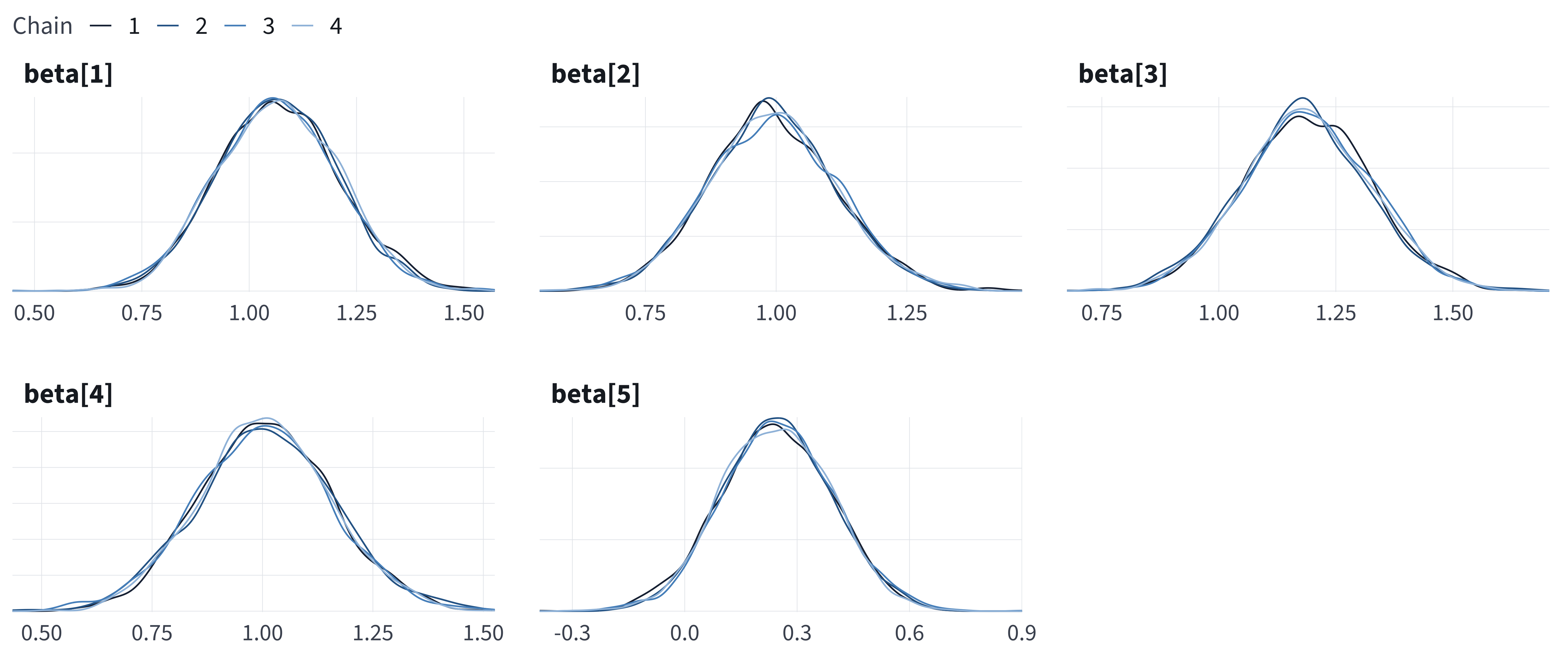
{bayesplot}: ridges

# ridges plot of densities of parameters
mcmc_areas_ridges(draws_beta)

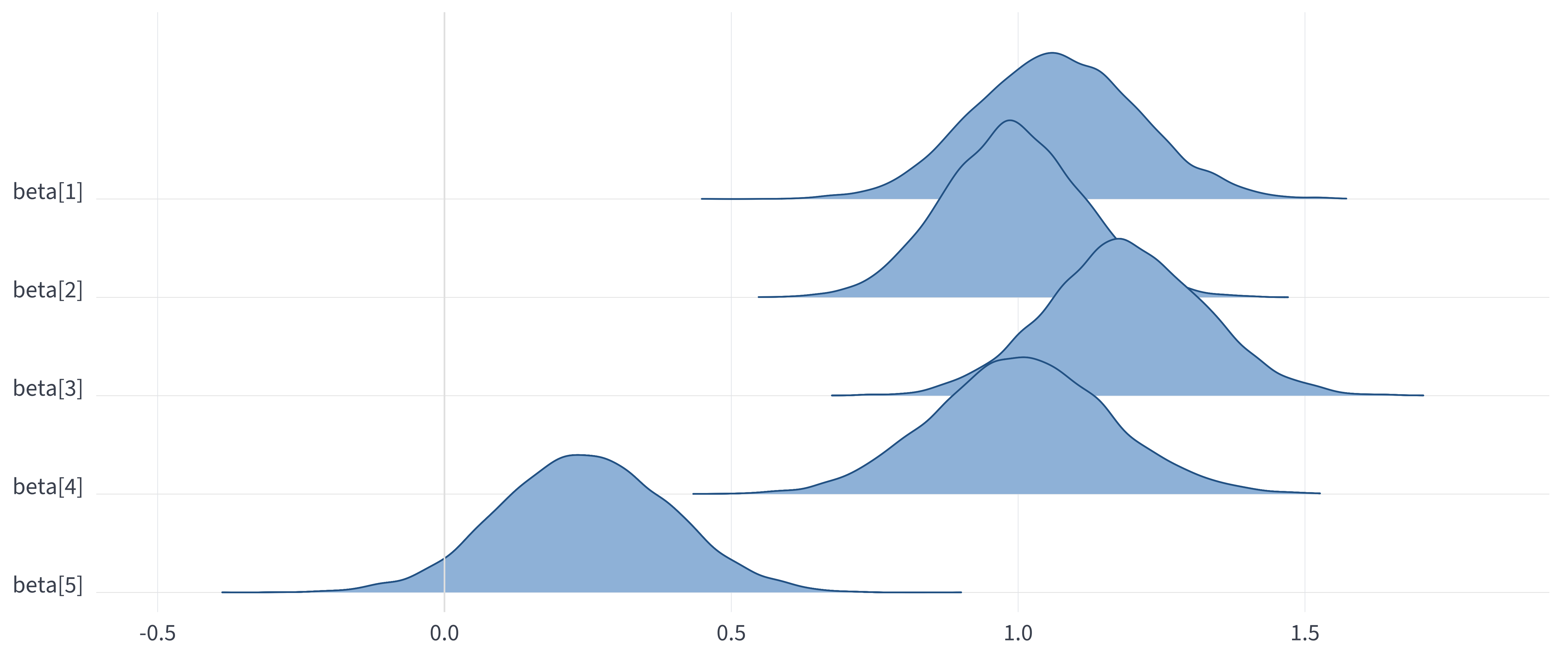
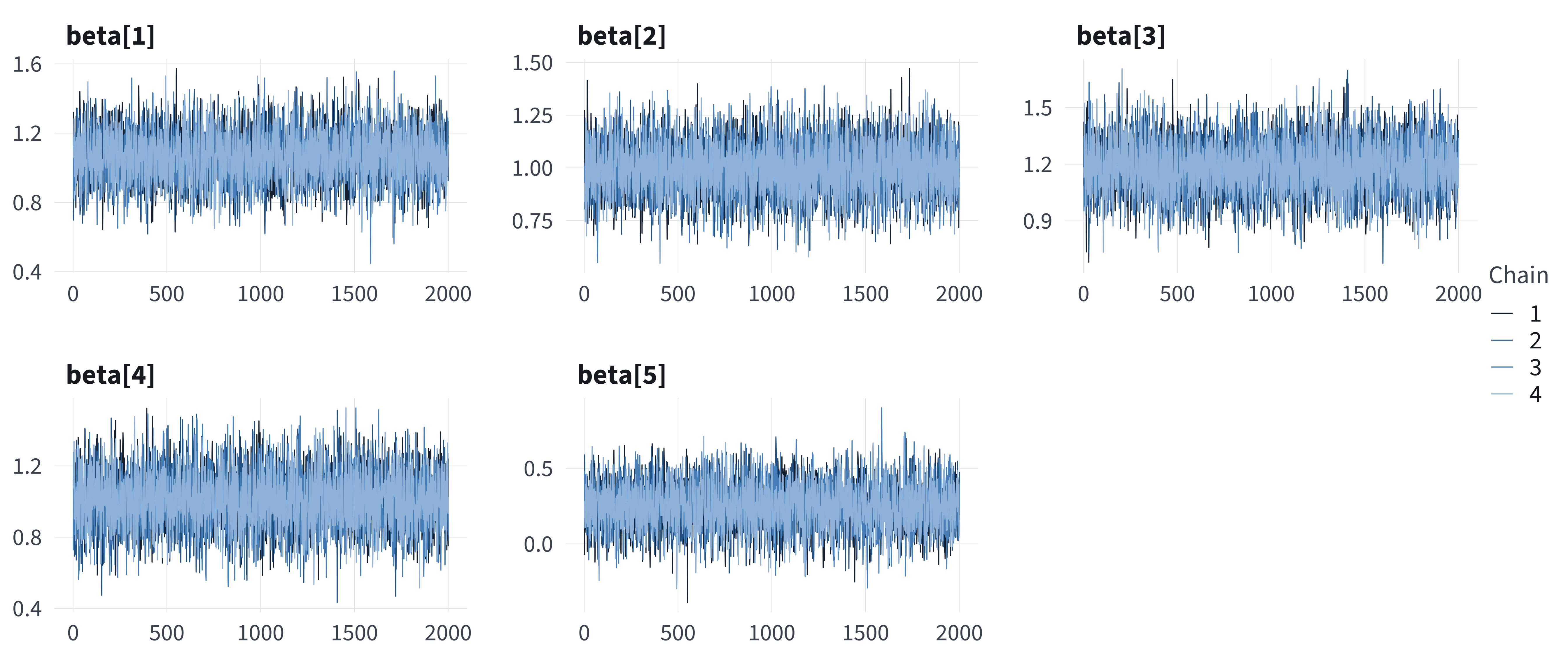
{bayesplot}: trace plots

# trace plots of parameters by chain
mcmc_trace(draws_beta)

ShinyStan

The ShinyStan app provides an interactive dashboard for convergence diagnostics, traceplots, divergences, and posterior summaries.

library(shinystan)

# launch the app for the {cmdstanr} fit
launch_shinystan(fit_cmd)

You can inspect trace plots, divergences, and other visual diagnostics interactively without additional coding.

Quantities of interest

# put the simulations of the coefficients into a matrix
beta_tilde <- fit_cmd$draws(variables = "beta", format = "draws_matrix")
head(beta_tilde)

# A draws_matrix: 6 iterations, 1 chains, and 5 variables
    variable
draw beta[1] beta[2] beta[3] beta[4] beta[5]
   1     1.1    0.93     1.1     1.1   0.125
   2     1.3    1.27     1.4     1.0  -0.071
   3     1.1    0.99     1.2     1.1   0.200
   4     1.1    0.93     1.0     1.1   0.076
   5     1.1    0.91     1.1     1.1   0.167
   6     1.0    0.79     1.0     1.1   0.335

Each row is one draw of \(\beta\), and each column is one coefficient.

First difference

To compute a first difference, transform draws using the invariance principle.

# make X_lo
X_lo <- cbind(
  "constant" = 1, # intercept
  "rs_age" = -0.5, # 1 SD below avg -- see ?arm::rescale
  "rs_educate" = 0,
  "rs_income" = 0,
  "white" = 1 # white indicator = 1
)

# make X_hi by modifying the relevant value of X_lo
X_hi <- X_lo
X_hi[, "rs_age"] <- 0.5  # 1 SD above avg

First difference

# function to compute first difference
fd_fn <- function(beta, hi, lo) {
  beta <- as.vector(beta)  # to prevent column/row confusion
  plogis(hi%*%beta) - plogis(lo%*%beta)
}

# transform simulations of coefficients into simulations of first-difference
fd_tilde <- numeric(nrow(beta_tilde))  # container
for (i in 1:nrow(beta_tilde)) {
  fd_tilde[i] <- fd_fn(beta_tilde[i, ], hi = X_hi, lo = X_lo)
}

# summarize: posterior mean, posterior SD, and 95% credible interval
mean(fd_tilde)

[1] 0.166

sd(fd_tilde)

[1] 0.02

quantile(fd_tilde, probs = c(0.025, 0.975))

 2.5% 97.5% 
0.127 0.206 

• The notes’ comments on the loop: for clarity, just do this one simulation at a time; i indexes the simulations.

Summary

Stan as modern MCMC
Stan automates MCMC using a hyper-optimized version of HMC. It efficiently samples from posteriors that are otherwise difficult to explore.

Interfaces
We run Stan from R with {cmdstanr}. The older {rstan} package runs the same Stan programs, but its summaries use older versions of R-hat and ESS.

Diagnostics and Visualization
Check \(\hat{R}\), ESS, and the HMC diagnostics (divergent transitions, maximum treedepth, E-BFMI). An R-hat larger than 1.01 or any divergent transitions after warmup mean that we cannot yet trust the draws. The $summary() and $diagnostic_summary() methods report these, and {bayesplot} and ShinyStan make it easy to explore them visually.

Stan and Metropolis

Stan generalizes what we learned with the Metropolis algorithm: the logic is the same, but the computation is vastly more efficient.

{brms}

{brms}

High-level interface to Stan
{brms} lets you specify Bayesian models using R’s familiar formula syntax y ~ x1 + x2, then translates them automatically into efficient Stan code for sampling.

Broad model support
It can fit all kinds of models. Much more general than any particular fitting function we’ve seen so far.

Seamless post-processing and visualization
Built-in tools integrate with {bayesplot}, {posterior}, and {tidybayes} to summarize, diagnose, and visualize posterior draws without writing any Stan code directly.

• Build note: Keynote “{brms}” slide (Fall 2025). Its line “This is worth emphasizing: {brms} writes efficient Stan code.” is left off the slide (it had an em dash).
• From the notes: The brm() function in {brms} takes glm()-like arguments, and writes accurate and fast Stan code.
• In-class script: https://pos5747.github.io/files/wk07-brms-logit.R

The turnout example

Here’s the syntax for our usual logistic regression model.

# load only the turnout data frame and hard-code rescaled variables
turnout <- ZeligData::turnout  |>
  mutate(across(age:income, arm::rescale, .names = "rs_{.col}"))

# formula
f  <- vote ~ rs_age + rs_educate + rs_income + race

# fit model with glm()
fit_glm <- glm(f, data = turnout, family = binomial)

# fit model with brm() via cmdstanr
fit_brm <- brm(f, data = turnout, family = bernoulli,
           chains = 4, cores = 4,
           backend = "cmdstanr",
           seed = 1234)

• [CTK: brm()’s default backend is still {rstan}; options(brms.backend = "cmdstanr") makes {cmdstanr} the default for the session]
• Build note: the notes use chains = 10, cores = 10; the deck uses 4 chains (and seed = 1234) to keep the render short.

glm() and brm()

glm() and brm() obtain the same estimates.

normalize_terms <- function(x) {
  x <- sub("^b_", "", x)  # brms to glm names
  x <- ifelse(x == "(Intercept)", "Intercept", x)  # unify intercept
  x
}

modelsummary(
  list("glm()" = fit_glm, "brm()" = fit_brm),
  coef_rename = normalize_terms,
  statistic = "conf.int",
  notes = "95% confidence intervals for glm(); 95% credible intervals for brm().",
  gof_map = "nobs"
)

	glm()	brm()
95% confidence intervals for glm(); 95% credible intervals for brm().
Intercept	1.058	1.063
	[0.787, 1.335]	[0.796, 1.346]
rs_age	0.993	1.002
	[0.758, 1.234]	[0.777, 1.245]
rs_educate	1.184	1.191
	[0.918, 1.456]	[0.932, 1.465]
rs_income	1.001	1.001
	[0.706, 1.308]	[0.706, 1.305]
racewhite	0.251	0.250
	[-0.039, 0.536]	[-0.048, 0.539]
Num.Obs.	2000	2000

• Build note: the notes’ table uses gof_map = NULL, which adds R2, AIC, BIC, Log.Lik., F, ELPD, LOOIC, WAIC, and RMSE rows; the slide keeps only Num.Obs. so the table fits.
• Footnote in the notes: The two are not mathematically equal, but they are very close here because {brms}’s default prior on the coefficients is flat. With flat or weak priors and this much data, it is rare that a Bayesian estimate or interval differs from the ML estimate or interval, outside of cases where maximum likelihood fails.

Diagnostics

{brms} warns only when an R-hat is larger than 1.05, so we check R-hat, ESS, and divergent transitions ourselves.

# R-hat and ESS for each parameter
summarise_draws(fit_brm, "rhat", "ess_bulk", "ess_tail")

# A tibble: 8 × 4
  variable      rhat ess_bulk ess_tail
  <chr>        <dbl>    <dbl>    <dbl>
1 b_Intercept  1.00     3909.    2745.
2 b_rs_age     1.000    3624.    3248.
3 b_rs_educate 1.00     4076.    3015.
4 b_rs_income  1.00     4158.    3321.
5 b_racewhite  1.00     4189.    2744.
6 Intercept    1.00     4028.    3083.
7 lprior       1.00     4028.    3083.
8 lp__         1.000    2012.    2690.

# number of divergent transitions after warmup
sum(nuts_params(fit_brm, pars = "divergent__")$Value)

[1] 0

{marginaleffects}

And {brms} plays very nicely with {marginaleffects}.

# compute first difference
comparisons(fit_brm, variables = list(rs_age = c(-0.5, 0.5)),
            newdata = datagrid(grid_type = "mean_or_mode"))

 Estimate 2.5 % 97.5 %
    0.167  0.13  0.206

Term: rs_age
Type: response
Comparison: 0.5 - -0.5

• For a {brms} fit, comparisons() reports the posterior median and an equal-tailed 95% credible interval, and no SE or SD column. get_draws() returns the posterior draws of the comparison, so any other summary is one line away (used for the table on the next slide).

Four routes to the same first difference

Method	Estimate	SE	2.5%	97.5%
First difference in Pr(vote) for rs_age from -0.5 to 0.5, other predictors at their means and race = white. glm() + comparisons(): ML estimate, delta-method standard error, and Wald 95% confidence interval. The other three rows: posterior mean, posterior SD, and 2.5th and 97.5th percentiles of the simulated first differences (for brm(), computed from get_draws(); comparisons() itself prints the posterior median and the same interval). metrop() uses a flat prior; Stan uses normal(0, 5) priors; brm() uses its defaults (flat on the coefficients).
glm() + comparisons(): ML + delta method	0.166	0.020	0.127	0.205
metrop(): posterior simulations	0.166	0.020	0.129	0.205
Stan: posterior simulations	0.166	0.020	0.127	0.206
brm() + comparisons(): posterior simulations	0.167	0.020	0.130	0.206

Four computations of one quantity. The ML route (last week’s tools) and the three posterior routes agree to the second decimal. Metropolis needed 80,000 draws (after burn-in) and a hand-tuned tau; Stan needed 8,000 and no tuning; brm() needed 8,000 and no Stan code. The small differences between the rows are Monte Carlo error plus the priors.

Expected values

# compute and plot expected values (i.e., predicted probabilities)
p <- predictions(fit_brm, variables = list(rs_age = seq(-1, 1, by = 0.1)),
            newdata = datagrid(grid_type = "mean_or_mode"))
ggplot(p, aes(x = rs_age, y = estimate, ymin = conf.low, ymax = conf.high)) +
  geom_ribbon(fill = "grey") +
  geom_line(color = lecture_colors[["blue"]])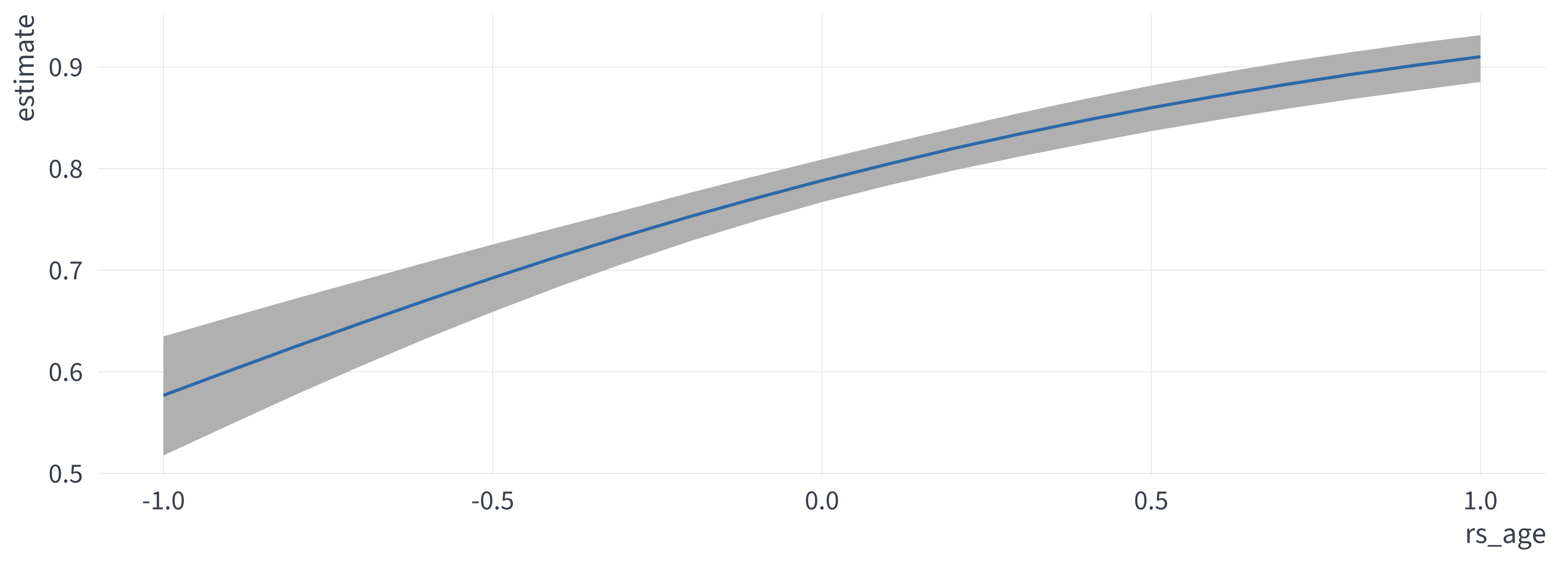

Modeling “smooth” relationships

To illustrate the power of MCMC and brm(), we can imagine fitting a smooth curve for age.

# smooth relationship between age and voting--notice the s()
f  <- vote ~ s(rs_age) + rs_educate + rs_income + race
smooth_fit <- brm(f, data = turnout, family = bernoulli,
           chains = 4, cores = 4,
           backend = "cmdstanr",
           control = list(adapt_delta = 0.99),  # avoids divergent transitions
           seed = 1234)

• From the notes: The details are not important for now, but this isn’t an easy task in our usual framework. But it’s straightforward with Bayesian MCMC via brm().
• [CTK: smooths often cause divergent transitions; with the default adapt_delta = 0.8 these two fits had 60 and 156 (of 10,000; CmdStan 2.40, seed = 1234); adapt_delta = 0.99 gives none with seed = 1234 (other seeds occasionally leave 1 of 10,000: 2 of 7 seeds checked)]
• Build note: those counts are from the notes’ 10-chain fits; the deck fits 4 chains, and both smooth fits here had 0 divergences.

Modeling “smooth” relationships

# compute and plot expected values (i.e., predicted probabilities)
p <- predictions(smooth_fit, variables = list(rs_age = seq(-1, 1, by = 0.1)),
            newdata = datagrid(grid_type = "mean_or_mode"))
ggplot(p, aes(x = rs_age, y = estimate, ymin = conf.low, ymax = conf.high)) +
  geom_ribbon(fill = "grey") +
  geom_line(color = lecture_colors[["blue"]])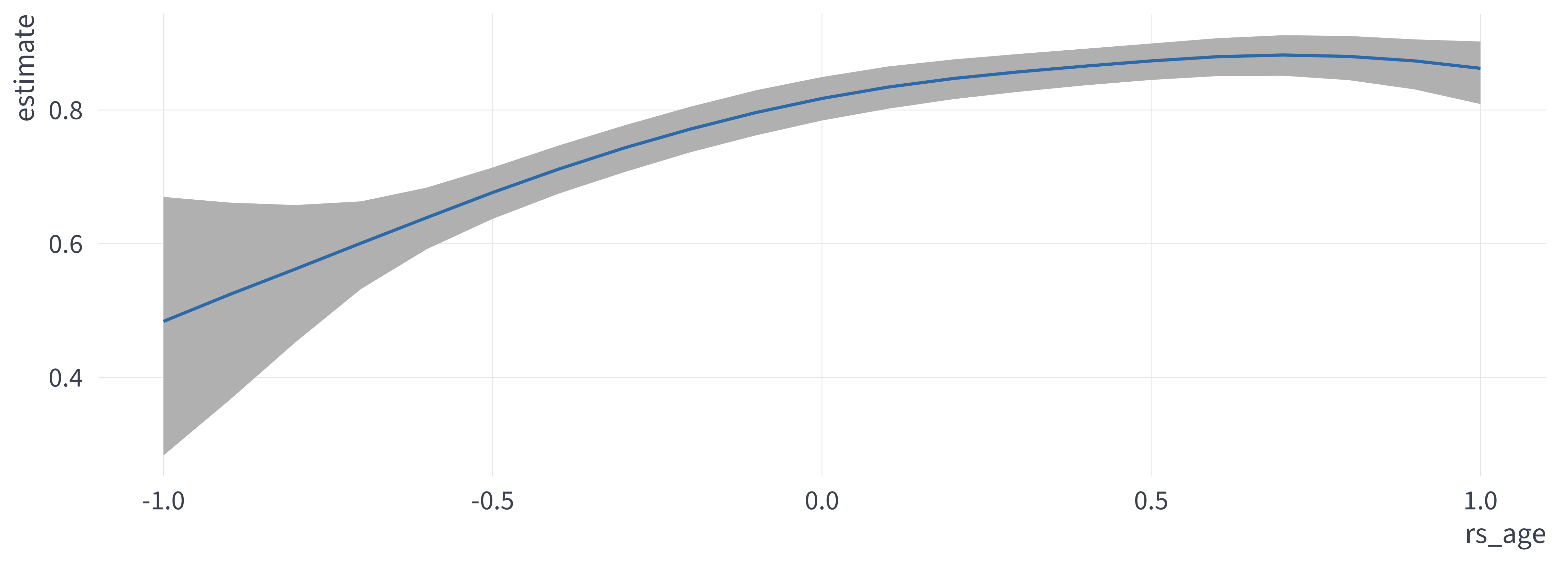

Awkwardly scaled variables

Also, brm() has no trouble with the variables on their original scales. The original scales pose a serious hurdle for our metrop() sampler.

# smooth relationship between age and voting--notice the s()
f  <- vote ~ s(age) + educate + income + race
smooth_fit <- brm(f, data = turnout, family = bernoulli,
           chains = 4, cores = 4,
           backend = "cmdstanr",
           control = list(adapt_delta = 0.99),  # avoids divergent transitions
           seed = 1234)

Awkwardly scaled variables

# compute and plot expected values (i.e., predicted probabilities)
p <- predictions(smooth_fit, variables = list(age = seq(18, 90, by = 1)),
            newdata = datagrid(grid_type = "mean_or_mode"))
ggplot(p, aes(x = age, y = estimate, ymin = conf.low, ymax = conf.high)) +
  geom_ribbon(fill = "grey") +
  geom_line(color = lecture_colors[["blue"]])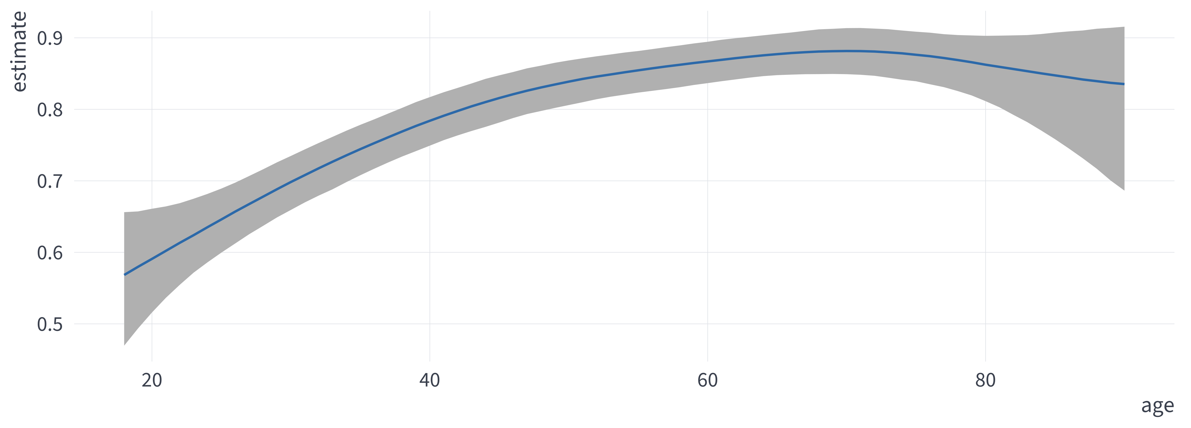

Use brm()

If brm() works for your application, you should much prefer it to writing your own Stan models.

LOOIC

Why not the AIC?

In Information Criteria, we compared Poisson and NB for Holland’s Santiago data with AIC and BIC. However, when we have posterior simulations, the AIC and BIC work poorly because we do not have a single point estimate. Instead, we have a distribution.

The AIC also works poorly with posterior simulations for two other reasons.

1. Plugging in a point estimate (e.g., the posterior mean) ignores the uncertainty in the posterior, while the LOOIC averages over all the draws.
2. The AIC’s penalty counts parameters, but a prior that pulls the estimates toward zero makes a model less flexible than its count of parameters suggests. With a strong prior or a hierarchical model, \(k\) overstates the model’s effective number of parameters.

When we have a sample from the posterior, we can instead use the LOOIC.

Example: Linear or cubic age?

First, the data and formulas.

# load only the turnout data frame and create rescaled columns
turnout <- ZeligData::turnout |>
  mutate(across(age:income, arm::rescale, .names = "rs_{.col}"))

# linear in age
f_linear <- vote ~ rs_age + rs_educate + rs_income + race

# cubic in age
f_cubic <- vote ~ rs_age + I(rs_age^2) + I(rs_age^3) +
  rs_educate + rs_income + race

Next fit the models.

fit_linear_brm <- brm(f_linear, data = turnout, family = bernoulli,
                      backend = "cmdstanr", chains = 4, cores = 4, seed = 1234)

fit_cubic_brm <- brm(f_cubic, data = turnout, family = bernoulli,
                     backend = "cmdstanr", chains = 4, cores = 4, seed = 1234)

When we have posterior simulations via Stan, we can use the LOOIC as an alternative to the AIC or BIC.

Compute the LOOIC

# looic for linear model
loo_linear_brm <- loo(fit_linear_brm)
loo_linear_brm

Computed from 4000 by 2000 log-likelihood matrix.

         Estimate   SE
elpd_loo  -1017.2 23.1
p_loo         5.3  0.2
looic      2034.4 46.1
------
MCSE of elpd_loo is 0.0.
MCSE and ESS estimates assume MCMC draws (r_eff in [0.8, 1.3]).

All Pareto k estimates are good (k < 0.7).
See help('pareto-k-diagnostic') for details.

# looic for cubic model
loo_cubic_brm <- loo(fit_cubic_brm)
loo_cubic_brm

Computed from 4000 by 2000 log-likelihood matrix.

         Estimate   SE
elpd_loo  -1011.4 23.3
p_loo         7.3  0.3
looic      2022.8 46.5
------
MCSE of elpd_loo is 0.0.
MCSE and ESS estimates assume MCMC draws (r_eff in [0.7, 1.5]).

All Pareto k estimates are good (k < 0.7).
See help('pareto-k-diagnostic') for details.

• elpd_loo (higher is better)
• p_loo (effective number of parameters)
• looic = −2 \(\times\) elpd_loo (lower is better)

Compare the two models

# compare the two models
loo_compare(loo_linear_brm, loo_cubic_brm)

          model elpd_diff se_diff p_worse diag_diff diag_elpd
  fit_cubic_brm       0.0     0.0      NA                    
 fit_linear_brm      -5.8     4.1    0.92                    

• loo_compare() prints the best model in the top row, and elpd_diff is relative to that best model.
• loo_compare() reports differences on the ELPD scale. ELPD differences are half the size of LOOIC differences and have the opposite sign (higher ELPD is better; lower LOOIC is better). Multiply by (−2) for the LOOIC scale (e.g., −5.8 elpd becomes 11.6 LOOIC).
• se_diff is the SE of the difference.

Some rules of thumb:

• For |elpd_diff| < 4, the models predict about equally well, regardless of se_diff.
• For |elpd_diff| > 4 AND large compared to se_diff: a meaningful difference (see ?loo-glossary).

The cubic model is ahead by 5.8 elpd with an se_diff of 4.1. This is modest evidence for the cubic.

From the chapter: It’s fine to use either. But the LOOIC connects nicely to the AIC and BIC, so that’s the one I’ve emphasized here.

From the chapter’s footnote: Compare Raftery’s table for BIC differences in Information Criteria, where we established “about 10” as a big difference between the models. Remember that LOOIC differences are twice elpd differences, so 4 elpd is the same as 8 LOOIC.

From the chapter’s aside: Raftery’s table in Information Criteria calls a BIC difference larger than 10 “very strong” evidence. The BIC, like the AIC and LOOIC, is on the \(-2 \times \log\) scale, so a BIC difference of 10 is the same size as a difference of 5 on the elpd scale.

The AIC and BIC, for comparison

# AIC and BIC from glm() fits, for comparison
fit_linear_glm <- glm(f_linear, family = binomial, data = turnout)
fit_cubic_glm  <- glm(f_cubic, family = binomial, data = turnout)
AIC(fit_linear_glm, fit_cubic_glm)

               df  AIC
fit_linear_glm  5 2034
fit_cubic_glm   7 2022

BIC(fit_linear_glm, fit_cubic_glm)

               df  BIC
fit_linear_glm  5 2062
fit_cubic_glm   7 2062

(The AIC is 2022.4 for the cubic and 2034.0 for the linear, and the BIC is 2061.6 and 2062.0.)

[CTK: the printed AIC/BIC tables round to whole numbers (options(digits = 3)); the caption gives one decimal.]

AIC and LOO

The AIC assumes the penalty, and LOO measures it.

Multinomial logit

The inverse-logit function

Suppose \(y_i \in \{0, 1\}\). Using logistic regression, we model \(\Pr(y_i = 1)\) as a function of covariates, so that

\[ \Pr(Y_i = 1) = \frac{\exp(X_i \beta)}{1 + \exp(X_i \beta)}. \]

The function \(f(z) = \frac{e^z}{1 + e^z}\) is called the inverse-logit function and maps any real number \(X_i \beta\) into a probability between 0 and 1.

Because the two probabilities must sum to one:

\[ \Pr(Y_i = 0) = 1 - \Pr(Y_i = 1) = \frac{1}{1 + \exp(X_i \beta)}. \]

The softmax function

The softmax generalizes the inverse-logit—it takes \(J\) real inputs (i.e., from \(\mathbb{R}^J\)) and scales them to sum to one.

\[ \text{softmax}(z_j) = \frac{\exp(z_j)}{\sum_{k=1}^{J} \exp(z_k)}, \qquad j = 1,\ldots,J. \]

Because the \(J\) outputs must sum to one, it is natural to interpret the outputs as probabilities.

The softmax function: \(J = 4\)

viewof sm_z1 = Inputs.range([-5, 5], {step: 0.1, value: -1,  label: "z1"});
viewof sm_z2 = Inputs.range([-5, 5], {step: 0.1, value: 1,   label: "z2"});
viewof sm_z3 = Inputs.range([-5, 5], {step: 0.1, value: 2,   label: "z3"});
viewof sm_z4 = Inputs.range([-5, 5], {step: 0.1, value: 0.5, label: "z4"});

// Softmax pieces
sm_labels = ["Pr(A)","Pr(B)","Pr(C)","Pr(D)"];
sm_zs = [sm_z1, sm_z2, sm_z3, sm_z4];
sm_exps = sm_zs.map(Math.exp);
sm_sumexp = sm_exps.reduce((a, b) => a + b, 0);
sm_ps = sm_exps.map(e => e / sm_sumexp);

// Data for stacked bar (one row, four segments)
sm_data = sm_ps.map((p, i) => ({ label: sm_labels[i], value: p, row: "softmax" }));

// === Two-column layout: sliders (left) + live table (right) ===
{
const container = html`<div style="
  display:flex;
  gap:24px;
  align-items:flex-start;
  padding-top:8px;
"></div>`;

// Left column: sliders
const left = html`<div style="display:grid; gap:10px; min-width:220px;"></div>`;
left.append(viewof sm_z1, viewof sm_z2, viewof sm_z3, viewof sm_z4);

// Right column: table
const rows = sm_labels.map((cls, i) => ({
Class: cls,
z: sm_zs[i],
"exp(z)": sm_exps[i],
Probability: sm_ps[i]
}));

const right = html`<div style="
  min-width:240px;
  max-width:560px;
  padding:4px 0;
  font-size:1.6rem;
  line-height:1.1;
"></div>`;

right.append(
Inputs.table(rows, {
columns: ["Class", "z", "exp(z)", "Probability"],
format: {
z: d => d.toFixed(2),
"exp(z)": d => d.toFixed(3),
Probability: d => (d * 100).toFixed(1) + "%"
}
})
);

container.append(left, right);
return container;
}

Plot.plot({
width: 940,
height: 200,
marginLeft: 20,
marginRight: 36,
marginBottom: 46,
x: {
domain: [0, 1],
tickFormat: d => (d * 100).toFixed(0) + "%",
label: null,
tickSize: 10,
tickPadding: 8
},
y: { axis: null },
style: {
fontSize: "22px",
fontFamily: "Source Sans 3, sans-serif"
},
color: {
legend: true,
label: "Class",
range: ["#e41a1c", "#377eb8", "#4daf4a", "#984ea3"],
swatchSize: 22,
style: { fontSize: "22px" }
},
marks: [
Plot.barX(
sm_data,
Plot.stackX({ x: "value", y: "row", fill: "label", sort: { fill: null } })
),
Plot.ruleX([0, 1])
]
})

Example inputs

Input z	Softmax p
-1	0.0303
1	0.2242
2	0.6095
0.5	0.1360

The OJS widget below allows you to experiment with \(J = 4\) inputs and see how the outputted probabilities change. (The widget needs the page served over http; the table on the right is the static fallback.)

Adding covariates

Now suppose the outcome takes \(J\) possible values:

\[ y_i \in \{1, 2, \ldots, J\}. \]

Example 1: We might label vote choice in the US as (1) abstain, (2) Republican, (3) Democrat, or (4) other.

Example 2: We might label coup attempts in a given country-year as (0) none attempted, (1) failed attempt, or (2) successful attempt.

Adding covariates

For each category \(j\), define a linear predictor \(\eta_{ij} = X_i \beta_j\). Here, each \(\beta_j\) is a vector of coefficients.

We can use the softmax function to convert these linear predictors into probabilities that sum to one.

\[ \Pr(Y_i = j) = \frac{\exp(\eta_{ij})}{\sum_{k=1}^{J} \exp(\eta_{ik})}, \qquad j = 1, \ldots, J. \]

This is a generalization of the inverse-logit to \(J\) categories. If \(J = 2\), the softmax reduces to the inverse-logit.

Identification

However, this model is not identified because adding any constant to each of the \(\eta_{ij}\) produces the same probabilities.

Example inputs

Input z	Softmax p
-1	0.0303
1	0.2242
2	0.6095
0.5	0.1360

Adding a constant (\(+2\))

New input z + 2	Softmax p
-1 + 2 = 1	0.0303
1 + 2 = 3	0.2242
2 + 2 = 4	0.6095
0.5 + 2 = 2.5	0.1360

Adding a constant to all inputs leaves the softmax unchanged. This is why the multinomial logit model requires an identification constraint.

Identification

To identify the model, we set \(\beta_J = 0\), so that \(\eta_{iJ} = 0\). Then for \(j = 1, \ldots, J-1\), we have

\[ \Pr(Y_i = j) = \frac{\exp(X_i \beta_j)} {1 + \sum_{k=1}^{J-1} \exp(X_i \beta_k)}. \]

And for the “baseline” category \(J\), we have

\[ \Pr(Y_i = J) = \frac{1} {1 + \sum_{k=1}^{J-1} \exp(X_i \beta_k)}. \]

Example: the 1992 presidential vote

• 1992 ANES; same respondents as the wk06 Bush approval example
• Outcome: vote_1992: Bush, Clinton, or Perot
• Predictors: party_id (−3 to 3), economy (1 = much better to 5 = much worse)

# load data; keep complete cases on the model's variables
vote <- read_csv("https://pos5747.github.io/data/bush-approval-1992.csv") |>
  select(vote_1992, party_id, economy) |>
  drop_na() |>
  mutate(vote_1992 = factor(vote_1992, levels = c("Bush", "Clinton", "Perot"))) |>
  glimpse()

Rows: 592
Columns: 3
$ vote_1992 <fct> Bush, Bush, Bush, Clinton, Clinton, Clinton, Bush, Bush, Bush, Bush, C…
$ party_id  <dbl> 2, 3, 3, 3, -2, -3, 2, 3, 2, 1, -3, -2, 3, 1, -1, -3, -1, -3, -3, -3, …
$ economy   <dbl> 4, 4, 3, 3, 5, 5, 4, 2, 4, 3, 5, 4, 4, 4, 5, 5, 4, 5, 4, 5, 4, 4, 5, 5…

[CTK: why Perot makes this nominal, not ordered]

[CTK: 592 voters complete on these variables]

[CTK: provenance: Adolph’s Problem Set 4; same file as the ordered example; Perot as the reason a nominal model is needed]

multinom()

# fit multinomial logit; first level (Bush) is the baseline
fit_vote <- multinom(vote_1992 ~ party_id + economy, data = vote, trace = FALSE)
summary(fit_vote)

Call:
multinom(formula = vote_1992 ~ party_id + economy, data = vote, 
    trace = FALSE)

Coefficients:
        (Intercept) party_id economy
Clinton       -1.98   -1.098   0.551
Perot         -1.52   -0.439   0.336

Std. Errors:
        (Intercept) party_id economy
Clinton       0.622   0.0856   0.151
Perot         0.585   0.0774   0.144

Residual Deviance: 870 
AIC: 882 

[CTK: two rows of coefficients, one linear predictor per non-baseline candidate; each relative to Bush]

[CTK: baseline first here (multinom()), last in the math above; the probabilities don’t change]

[CTK: signs: party_id negative for both rows (Republicans → Bush); economy positive for both (worse economy → away from Bush)]

Probabilities with {marginaleffects}

# probability of each candidate as party ID varies
p_vote <- predictions(
  fit_vote,
  newdata = datagrid(party_id = -3:3),
  type = "probs")

# colors follow the factor levels:
# Bush, Clinton, Perot
ggplot(p_vote,
       aes(x = party_id, y = estimate,
           ymin = conf.low, ymax = conf.high,
           color = group, fill = group)) +
  geom_ribbon(alpha = 0.2, color = NA) +
  geom_line() +
  scale_color_lecture() +
  scale_fill_lecture() +
  labs(x = "Party ID", y = "Probability",
       color = "Candidate", fill = "Candidate")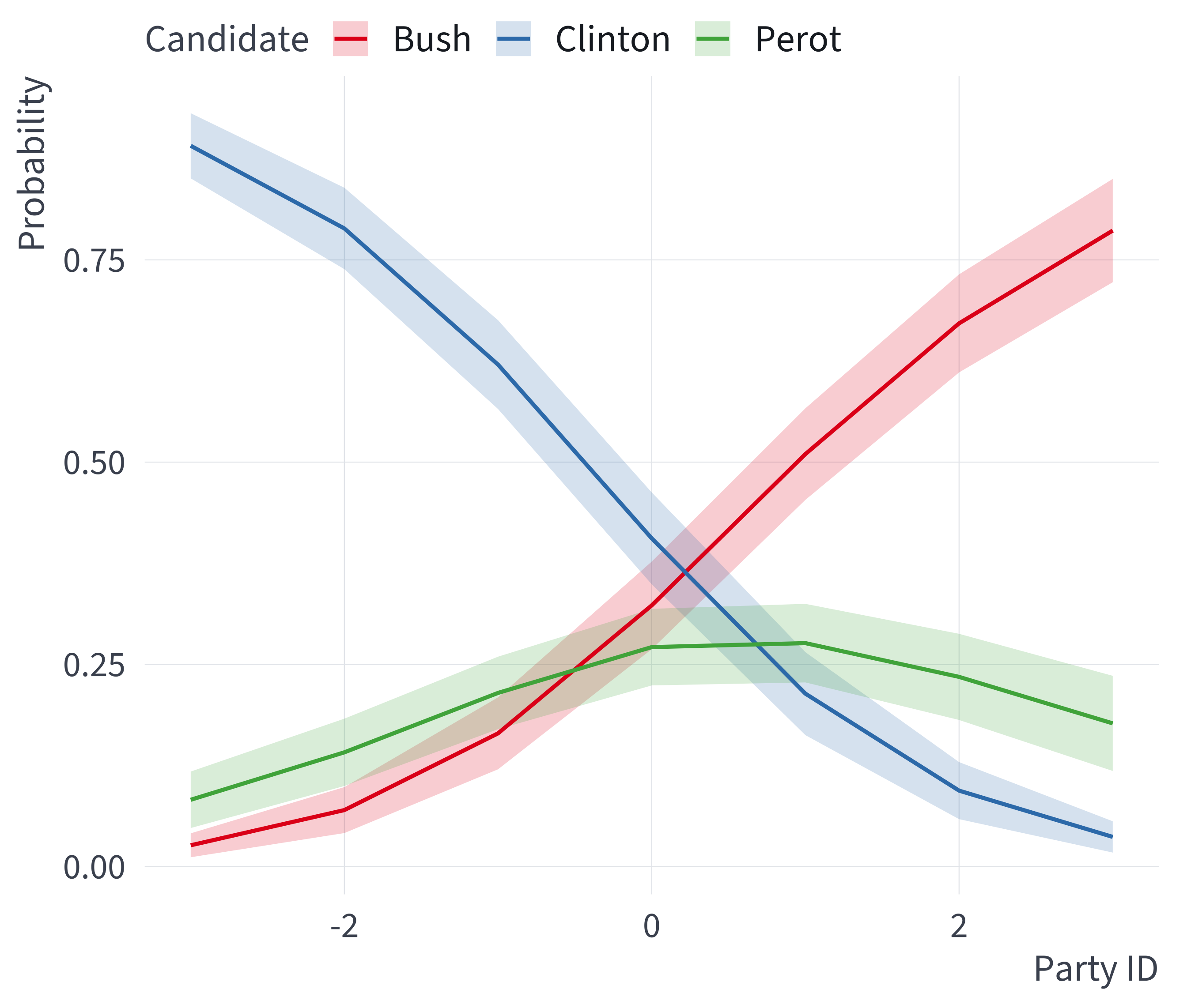

[CTK: Pr(Perot) rises then falls (about 0.08 at −3, peak about 0.28 at 0 to 1, 0.18 at 3), though both linear predictors are linear in party ID]

[CTK: why: Perot’s party_id coefficient (−0.44) sits between Bush’s (0) and Clinton’s (−1.10); the softmax shares probability]

[CTK: so the sign of a coefficient doesn’t give the direction of that category’s probability; compute probabilities]

First differences

# change in each candidate's probability as the economy goes from
# "better" (2) to "worse" (4), for a typical respondent
comparisons(fit_vote,
            variables = list(economy = c(2, 4)),
            newdata = datagrid(grid_type = "mean_or_mode"),
            type = "probs") |>
  as_tibble() |>
  select(term, contrast, group, estimate, conf.low, conf.high)

# A tibble: 3 × 6
  term    contrast group   estimate conf.low conf.high
  <chr>   <chr>    <fct>      <dbl>    <dbl>     <dbl>
1 economy 4 - 2    Bush     -0.219   -0.342    -0.0958
2 economy 4 - 2    Clinton   0.180    0.0874    0.272 
3 economy 4 - 2    Perot     0.0389  -0.0508    0.129 

[CTK: worse economy: Bush −0.22, Clinton +0.18, Perot +0.04 (CI includes 0)]

[CTK: Perot’s economy coefficient is positive (0.34), but Clinton gains most of what Bush loses]

brm()

# fit the same model with brm(); categorical() is the multinomial logit,
# with the first level (Bush) as the baseline
fit_vote_brm <- brm(vote_1992 ~ party_id + economy,
                    data = vote,
                    family = categorical(link = "logit"),
                    backend = "cmdstanr",
                    chains = 4,
                    cores = 4,
                    seed = 1234)

brm() vs. multinom()

	multinom()		brm()
Term	Estimate	SE	Estimate	SE
multinom(): ML estimates and standard errors. brm(): posterior means and standard deviations.
Clinton	Clinton	Clinton	Clinton	Clinton
Intercept	-1.978	0.622	-1.987	0.623
party_id	-1.098	0.086	-1.112	0.085
economy	0.551	0.151	0.554	0.151
Perot	Perot	Perot	Perot	Perot
Intercept	-1.519	0.585	-1.539	0.591
party_id	-0.439	0.077	-0.445	0.079
economy	0.336	0.144	0.341	0.146

Table code: compare_mnl() and tt_mnl() in the notes (Multinomial Logit, With brm())

[CTK: posterior means within about 0.02 of the ML estimates (e.g., Clinton party_id −1.11 vs −1.10; Perot economy 0.34 vs 0.34); default priors barely matter at N = 592]

brm() + {marginaleffects}

# for brms categorical fits (and only those), predictions()
# drops the newdata columns and returns rowid + group, so
# build the grid first and join party_id back by rowid
grid_vote <- datagrid(model = fit_vote_brm,
                      party_id = -3:3)
p_vote_brm <- predictions(fit_vote_brm,
                          newdata = grid_vote) |>
  left_join(select(grid_vote, rowid, party_id),
            by = "rowid")
ggplot(p_vote_brm,
       aes(x = party_id, y = estimate,
           ymin = conf.low, ymax = conf.high,
           color = group, fill = group)) +
  geom_ribbon(alpha = 0.2, color = NA) +
  geom_line() +
  scale_color_lecture() +
  scale_fill_lecture() +
  labs(x = "Party ID", y = "Probability",
       color = "Candidate", fill = "Candidate")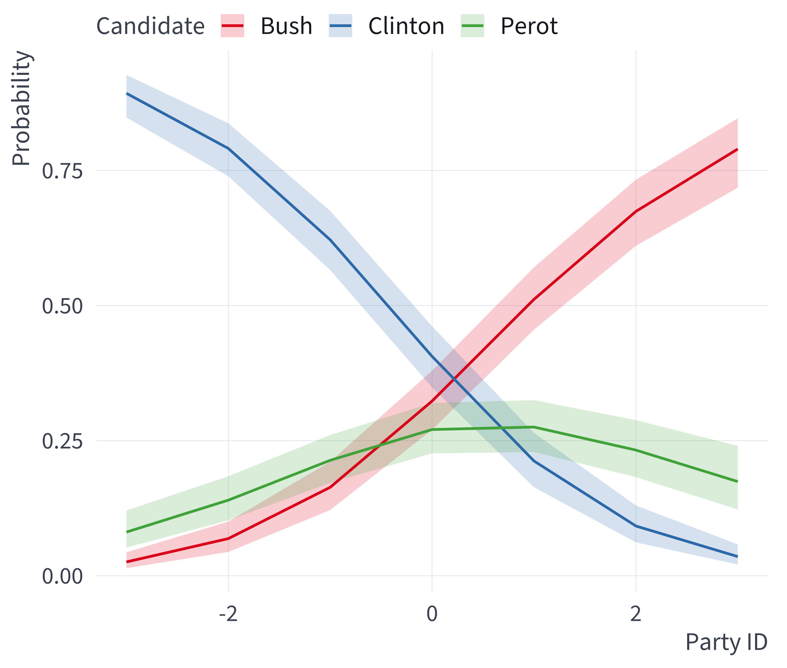

[CTK: same {marginaleffects} code, no type = "probs"; group column holds the candidate; the grid columns need joining back by rowid]

Checked 2026-10-06 (marginaleffects 1.0.0): the same call on the multinom() fit and on a brms bernoulli fit returns the grid columns; only the brms categorical fit drops them. A marginaleffects quirk, not a brms one; an investigation prompt was written for Carlisle.

[CTK: why bother with brm(): priors, hierarchical extensions (weeks 10–11)]

Another example: Balancing the federal budget

# 2012 CCES; "Raise taxes" first, so it is the baseline
cces <- read_csv("https://pos5747.github.io/data/cces2012-budget.csv") |>
  mutate(budget = factor(budget, levels = c("Raise taxes",
                                            "Cut defense spending",
                                            "Cut domestic spending")))

# fit multinomial logit; party ID from 1 (strong Democrat) to 7 (strong Republican)
fit_budget <- multinom(budget ~ party_id + female + income, data = cces, trace = FALSE)

# probability of each choice as party ID varies
p_budget <- predictions(fit_budget, newdata = datagrid(party_id = 1:7), type = "probs")

This example is inspired by a SAGE Research Methods Datasets guide (Reid 2020).

Another example: Balancing the federal budget

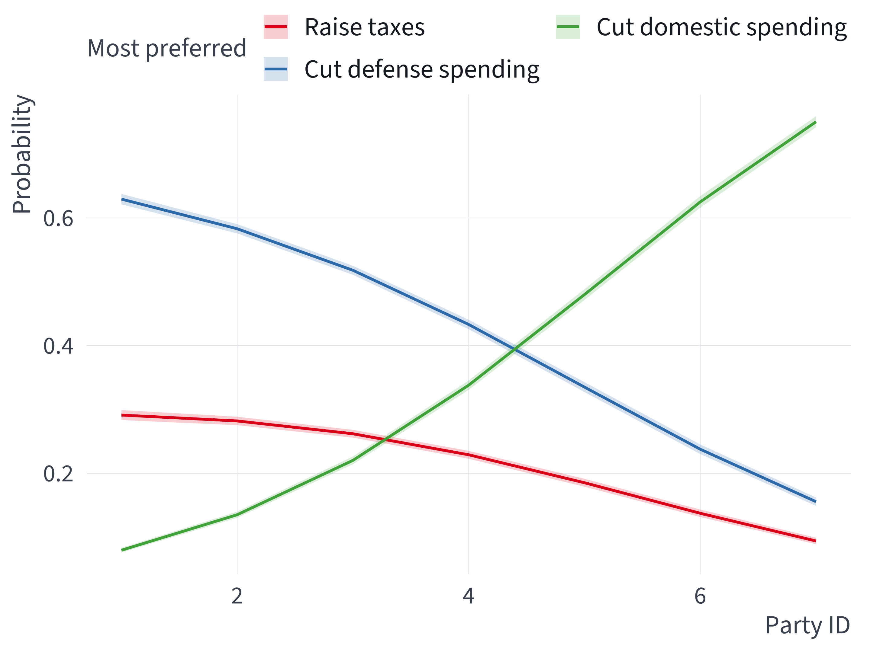
• 2012 CCES; 45,237 respondents
• Three categories: cut defense spending, cut domestic spending, or raise taxes.
• female at its mode (1) and income at its rounded mean (6, $50,000–59,999).
• Strong Democrats to strong Republicans: Pr(cut domestic spending) 0.08 to 0.75; Pr(cut defense spending) 0.63 to 0.16; Pr(raise taxes) 0.29 to 0.09.

Model: multinom(budget ~ party_id + female + income, data = cces); party ID from 1 (strong Democrat) to 7 (strong Republican). This example is inspired by a SAGE Research Methods Datasets guide (Reid 2020).

brm() fits every model we’ve seen so far

Model	ML	brm(family = ...)
Normal (linear)	lm()	gaussian()
Logit	glm(family = binomial)	bernoulli()
Poisson	glm(family = poisson)	poisson()
Negative binomial	MASS::glm.nb()	negbinomial()
Zero-inflated NB	glmmTMB::glmmTMB()	zero_inflated_negbinomial()
Ordered logit	MASS::polr()	cumulative(link = "logit")
Multinomial logit	nnet::multinom()	categorical()

We can use brm() to fit all the models we’ve seen so far in the course.

[CTK: wk06’s polr() fit works as brm(family = cumulative("logit")), same parameterization (cutpoints = Intercept[j]); this slide replaced the two-slide ordered callback 2026-10-06]

[CTK: why bother with brm(): priors, hierarchical extensions (weeks 10–11)]

Ordered vs. nominal

Ordered

cumulative()

one set of coefficients

Nominal

categorical()

\(J - 1\) sets

[CTK: ordered (cumulative()) vs nominal (categorical()): one set of coefficients vs J − 1 sets; Red State Part 3 in the exercises (did not vote / Harris / Trump, an unordered outcome)]

Wrap

Why MCMC?

MCMC

MCMC offers a powerful and general way to sample from an unnormalized (log-)posterior. The Metropolis algorithm is one such method. Hamiltonian Monte Carlo (HMC) via Stan is even better.

R-hat and burn-in

The first MCMC samples are highly dependent on the starting values. Because of this, you need to:

1. Discard the samples from a burn-in period.
2. Run multiple chains and check that R-hat is less than 1.01.

ESS and large samples

The MCMC samples are dependent on the previous samples. Because of this, you need to:

1. Generate more samples than you would need if they were independent.
2. Use ESS to understand your effective sample size.

From the Summary of the Metropolis chapter: “There are three important points in this chapter.” Read the exit ticket against these three.

This week’s exercises

1. Three samplers, one posterior
2. brm()
3. Convergence
4. brm() arguments
5. Experimenting with difficult posterior
6. Perot
7. Red State, Blue State: Part 3
8. Polynomials in age and the LOOIC

Solutions open Fri Oct 9, noon · No weekly assessment next week: midterm Tue Oct 13

Midterm

• Tue Oct 13
• Weeks 1–7
• Closed book

Exit ticket

List three important ideas from today’s class. For each, briefly connect it to one or more ideas from last week.